Brown University School of Engineering

ENGN 2502 3D Photography / Assignment 4

Spring 2016

• 3DP 2016 Home
• Assignments

Build Your Own Laser 3D Scanner

Downloads

Download the new course software source files 3dp-course-2016-assignment4-1.0.zip . Remember to copy your homework1.hpp, homework1.cpp, homework2.hpp, homework2.cpp, homework3.hpp and homework3.cpp files into the src/homework directory.

Hardware

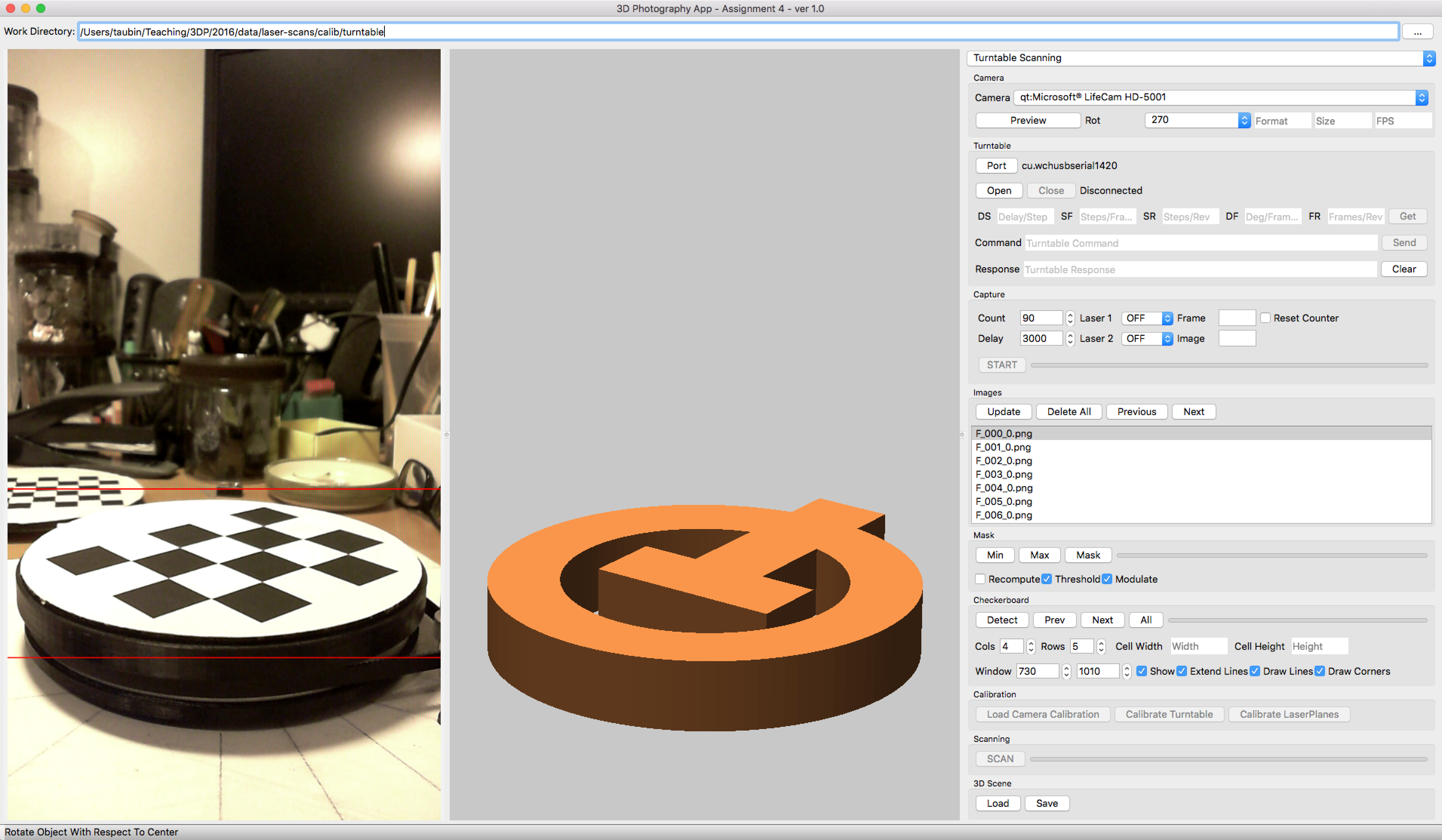
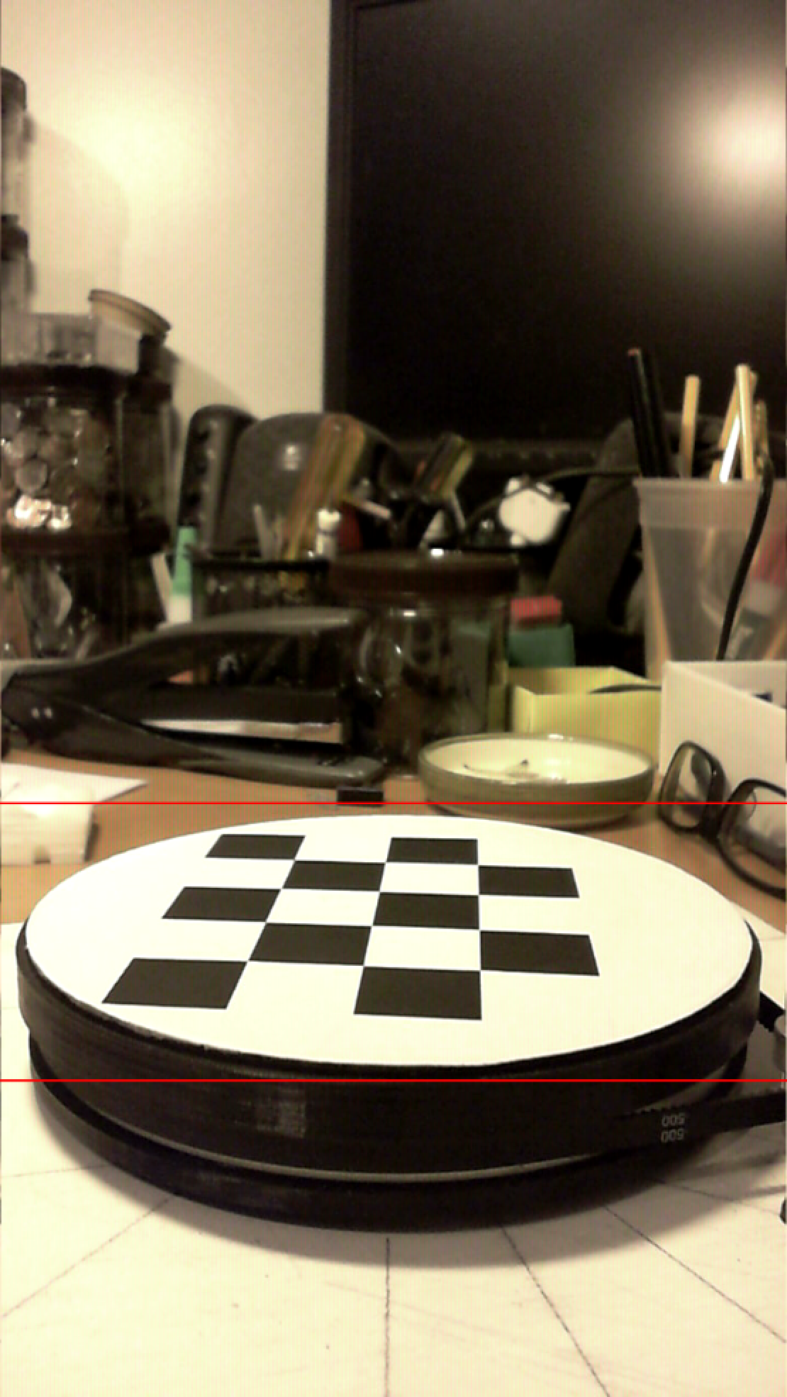
The picture above shows one of four similar low cost 3D scanners that we have fabricated for this assignment. This 3D scanner is controlled by the course software running in your computer. The scanner is connected to the computer through two USB ports. One of these ports is used to connect the built-in camera, which your computer showld recognize as a regular USB camera. The second USB port is used to connect the scanner controller to the computer. The course software communicates with the scanner controller through a serial port. The Hardware Fabrication page contains instructions to fabricate a copy of this scanner, including the STL files used to fabricate the 3D printed parts. This scanner is constructed on a 10 inch x 12 inch piece of plywood. It comprises: 1) a ball-bearing turntable, belt-driven by a stepper motor; 2) a USB camera; 3) two red laser line generator moduless; 4) a control board; and 5) a number of simple 3D printed parts which are used to atach the various components to the plywood board. The control board, which was built on a prototyping printed circuit board, contains an Arduino Nano microcontroller, a stepper motor driver board, and a few electronic components necessary to be power the laser modules and to able to turn them on and off under computer control. The USB port in the Arduino Nano is used to connect the controller board to the computer. The Arduino, the laser modules, and the stepper motor are all powered by the computer through the USB.

Arduino Software

The Arduino Nano in each of the four 3D scanners runs one of the following sketches Turntable-TB6612FNG-1.ino.zip, Turntable-TB6612FNG-2.ino.zip, Turntable-TB6612FNG-4.ino.zip, or Turntable-TB6612FNG-5.ino.zip. Except for I/O pin assignments, which are different in the four scanners, the four sketches are identical. The sketches are already installed in the Arduinos.

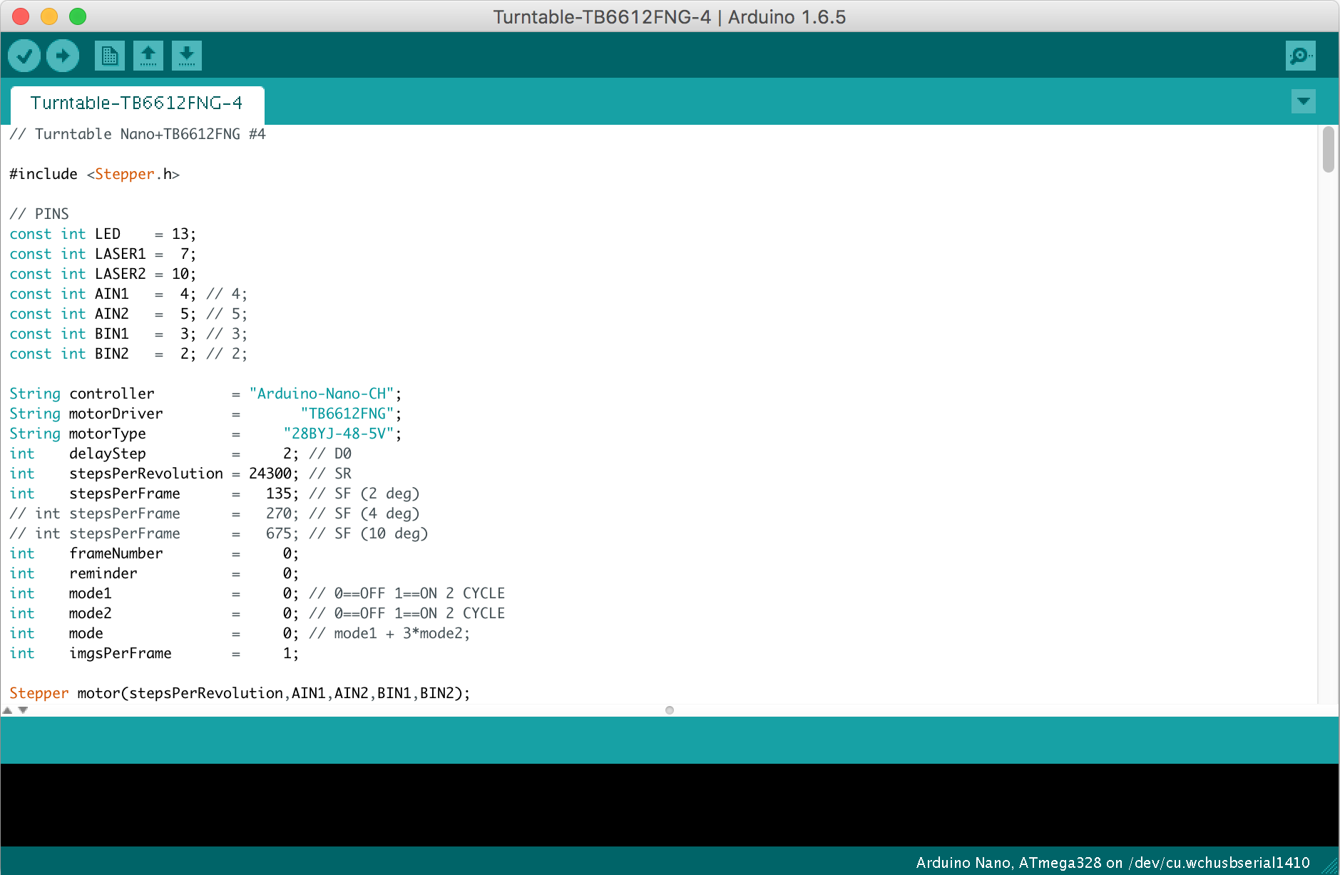
The Arduino Nano board, as well as other Arduino models, contains a USB/Serial chip, since the microcontroller itself does not have native support for USB. When you connect the Arduino to your computer through a USB port, your computer may or may not recognize the USB/Serial device. It it does not recognize the device you will have to install the proper driver in your computer before you can continue. We have used a low cost Chinese Arduino Nano clone in these scanners, which uses the CH340G USB/Serial chip. Sources for the driver are easy to find in the Internet, such as in this web page . Once your computer recognizes the device, the course software should be able to establish a communication link with the Arduino, and it should be able to control the turntable.

3D Scanner Software

A new Turntable Scanning panel has been added to the course software to implement this assignment. The GUI is composed of three windows. The left window shows images. The center window shows a 3D scene, and the right window is the control panel.

Camera

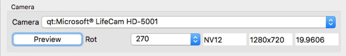
The first step is to be able to capture images within the course software using the 3D scanner camera. You should connec the 3D scanner camera to your computer before you launch the course software, because the software makes a list of available cameras only at start-up. Then you should select the 3D scanner camera from the list of available cameras. We have used "Microsoft LifeCam HD-5000" or "Microsoft LifeCam HD-5001" cameras in the construction of these scanners, on one hand because they are very small and light, and on the other hand because we had several available from a previous project. These cameras have a native resolution of 1280x720 pixels, and they are mounted so that the long axis is vertical, as shown in the previous picture. To make the software display the images in the proper orientation, you should select 270 as the Rotation value. If you press the "Preview" button, the software should display live video from the camera.

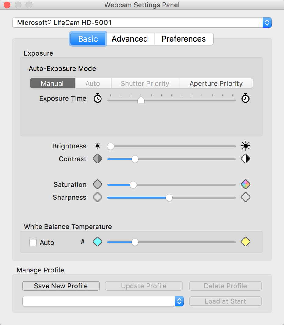
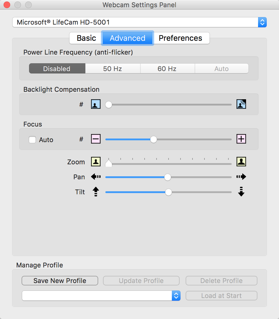
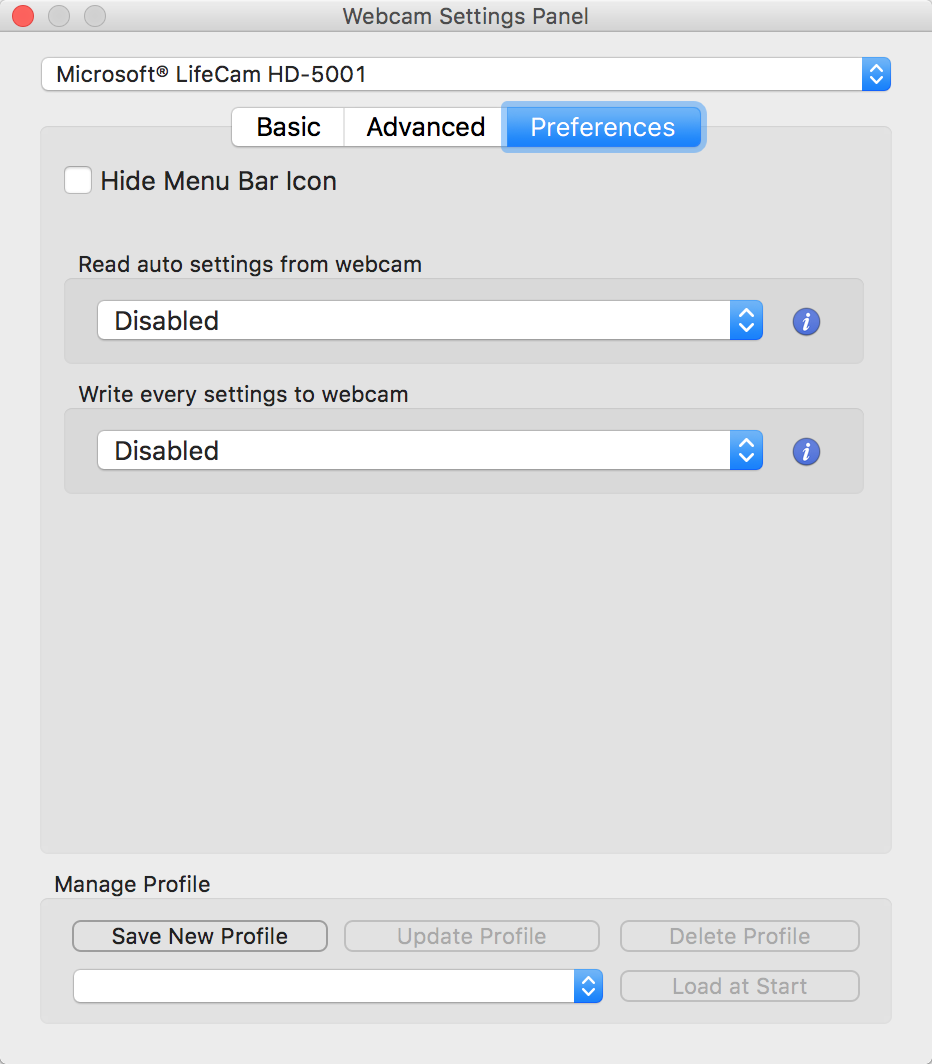
These are cameras with auto-focus functionality. A number of other parameters are also automatically set, and most camera drivers let the camera adjust those parameters dynamically. You will need to locate camera driver software which should allow you to disable all the automatic settings and to set camera parameters. We cannot allow the parameters to change, since changing the parameters affects all our calibration routines, as well as the image processing algorithms. For example, I am using an app named "Webcam Settings" which serves this purpose for my machine running OSX. There are similar applications for Windows and for other operating systems. The application should run in parallel with the course software so that you can adjust the parameters while the course software is displaying the camera video in preview mode.

Turntable Control

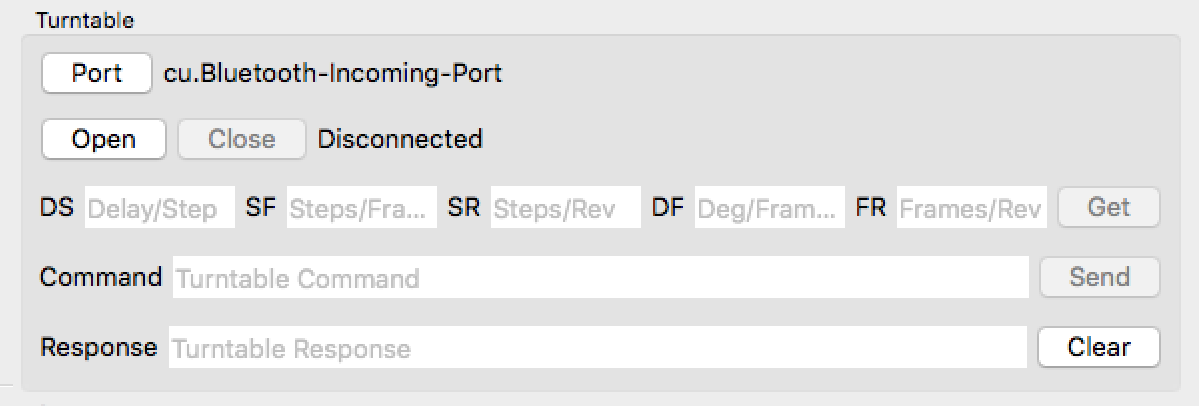
The next step is to establish communication with the turntable controller, and to verify that the software is able to control the turntable. Connect the Arduino to the computer through a serial port. Verify that the computer recognizes the USB device. Again, you should do this before starting the course application. Then, in the Turntable panel press the "Port" button.

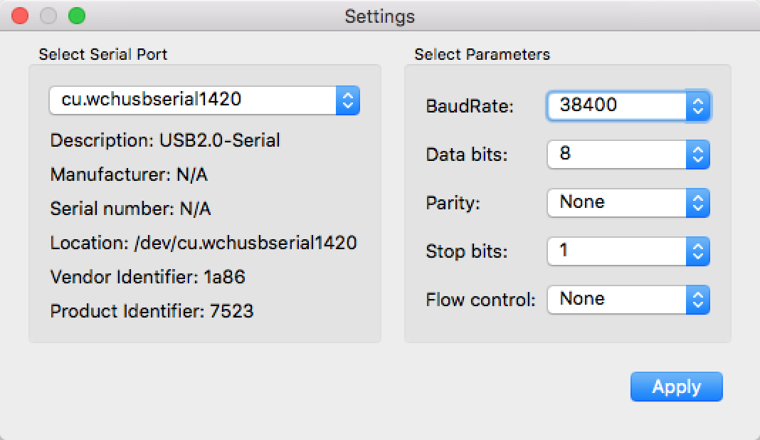
The following dialog window should pop-up. In this dialog you should be able to select the proper serial port and the serial port communication parameters: Baud Rate = 38400, Data Bits = 8, Parity = None, Stop Bits = 1, Flow Control = None. After you make your selections press the "Apply" button.

Back into the "Turntable" group, press the "Open" button to try to establish the communications link with the turntable controller. If successful, the "Open" button should be disabled, "Close" button should be enabled, and the communication parameters should be visible next to the "Close" button

The turntable controller software stores a number of parameteres which can be retrieved, and subsequently modified. After the connection is established, press the "Get" button. A few seconds later all the fields to the left of the "Get" button should be updated with numerical values. If they are not, press the "Get" button again. The DS parameter measures Delay per Step in miliseconds. This is the length of the pulses sent by the Arduino to the stepper motor to make it move, and determined the speed of motion. It is not advisable to change this value. In this assignment we wil refer to a "Frame" as a group of images captured with the turntable at a fixed position. A frame could be composed of 1 to 3 images, depending on whether the lasers are turned on, or not. If the lasers are kept off at all times, which we will need to calibrate the turntable, every frame would comprise a single image. The SF parameter measures the number of stepper motor Steps per Frame. The SR parameter measures the number of stepper motor Steps per Revolution. The last two parameters are computed from the previous two. The FR parameter, which measures the number of Frames per Revolution, is computed as the number of steps per revolution divided by the number of steps per frame, i.e. as SR/SF. Finally, the parameter DF, which measures the number of Degrees per Frame, is computed as 360 divided by the number of frames per revolution, i.e. 360/FR.

Even though the number of steps per revolution of the motor is well known from the motor specifications, the fact that the motor has a built-in speed reduction gearbox, that the motor is connected to the turntable through a belt, and that the motor has a belt pulley but the turntable ball-bearing does not have teeth, it is quite difficult to determine the number of steps per revolution as a result of a computation. It is advisable to develop an image-based method to measure the number of steps per revolution. Once it is determined, it can be stored in the Arduino controller by editing the SR field and pressing the Enter key in your keyboard. For example, the following picture shows the result of changing the parameter SR from the default 24300 to 24500. The computed values of DF and FR are updated as well.

The Arduino controller will remeber this value while it is powered on through the USB cable, but will forget it as soon as the cable is disconnected. To make it persists, the value should be updated in the Arduino sketch, and the sketch should be reloaded into the Arduino within Arduino IDE. Since this value is a function of the specific scanner hardware configuration, and it is not expected to change over time, it is a good idea to calibrate it precisely.

In addition to the value of SR, the values of DS and SF can be modified as well, by editing the value and pressing return. These changes are only allowed while the software is connected to the turntable controller, since otherwise the changes cannot be transmitted. Again, the modified values will persist while the Arduino is powered through the USB cable. Closing and reopening the serial port should not change these values. The values will revert to those stored in the Arduino sketch as soon as the Arduino is powered off. To make the changes permanent the values should be updated in the Arduino sketch, and the sketch should be reloaded into the Arduino within Arduino IDE.

The software communicates with the Arduino through the serial port using a simple text-based protocol defined in the Arduino sketch. If you know the protocol, you can type a command in the "Command" line and press the "Send" button to send it to the Arduino. The Arduino will then execute the comand and send another string as the response. The response is ususally just "OK", but some commands result in longer responses.

It is not necessary to describe the protocol here, since you will not have to use most of them directly. Again, the protocol is defined in the Arduino sketch, and it comprises a small number of commands. The only commands that might be useful to know are those which control the lasers, as well as those which make the turntable move by one frame or one revolution: "M 0" turns the two lasers off; "M 1" turns the left laser on and the right laser off; "M 3" turns the left laser off and the right laser on; "M 4" turns the two lasers on; "FF" and "BF" move the turntable forward and backward by one frame; and "FR" and "BR" move the turntable forward and backward by one revolution.

Image Capture

As in previous assignments, before you start capturing images, you need to a directory structure to save the images to be captured, as well as other files to be created, in an organized fashion. In fact, you will need at two or three different directories to store the images that you will use to calibrate the camera, the turntable, and the laser planes, and then one additional directory to store the images to be captured while scanning each object. For example, I created a directory named "/Users/taubin/Teaching/3DP/2016/data/laser-scans" as the top directory for this 3D scanner. Then I created a subdirectory of "laser-scans" named "calib", and three subdirectories of "calib" named "camera", "turntable", and "laser". Later on, for each scanning session I will create a subdirectory of "laser-scans" appropriately named. You may decide to use a different directory structure, but you need to remember to switch to the proper directory for each step of the calibration process, and later for each scanning session. If you do not switch directories, then the images that may exist in the work directory may be overwritten, and you may have to redo previous steps.

The software provide means to automate the process of image capture and turntable control. In the Capture group select the number of frames to be captured using the "Count" parameter. When the software is started, the frame counter is initialized to 0. The frame counter is increased after each image is captured. The "Reset Counter" checkbox determines whether or not the frame counter is reset before the next capture sequence. Whether the "Reset Conter" checkbox is checked or not, the software does not check whether or not the file name to be used to save each image corresponds to an existing file. If the file exists, the software will silently overwrite it.

Each frame is composed of between one and three images, depending on the setting you select for the lasers. For each one of the two lasers, you can specify that the laser be kept off all the time, on all the time, or cycle. If both lasers are always off or always on, the each frame is composed of one image. If one laser is specified to be always on or always off, and the other laser is specified to be cycling, then each frame will be composed of two images, where the first laser is always on or off, as specified, and the second laser is on in one image, and off in the other. If both lasers are specified to be cycling, then each frame is composed of three images, the first image with both lasers off, the second image with the first laser on and the second laser off, and a third image with the first laser off and the second laser on. The software takes care of sending the proper commands to the turntable and to capture the images at the proper times to automate the process.

During each capture sequence, the frame number and the image number within the frame is displayed, while the corresponding image is captured, and the progress bar located next to the "Stop" button shows in analog form the progress towards the end of the capture sequence.

Since the communication through the serial port between the computer and the Arduino is not very reliable, the software has to apply certain delay. For example, when the software sends a command to the Arduino requesting the turntable to advance by a certain number of steps, the Arduino may send a response back to the computer before the mechanical action has been completed. If the computer sends another command at that time, the Arduino may just ignore it. You can specify this parameter in the "Delay" field. The default value for this parameter, 2000 ms, works well with the default turntable parameters stored in the Arduino sketch. If you reduce the number of frames per revolution, increase this value inversely proportionately and test the motion.

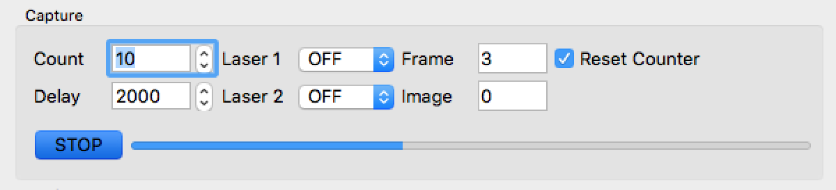
If you start a long sequence, and you need to stop it, perhaps because you started the sequence with the wrong parameters, you can always press the "STOP" button, change the parameters and start again. Kep in mind, though, that if the "Reset Counter" checkbox is not checked, the first frame of new sequence will start after the last frame captured in the aborted sequence, and all the frames capture during the aborted sequence will remain in the work directory. On the other hand, if the "Reset Counter" checkbox is checked, the frame counter will be reset to 0, and files existing in the work directory with the new frame names will be overwritten.

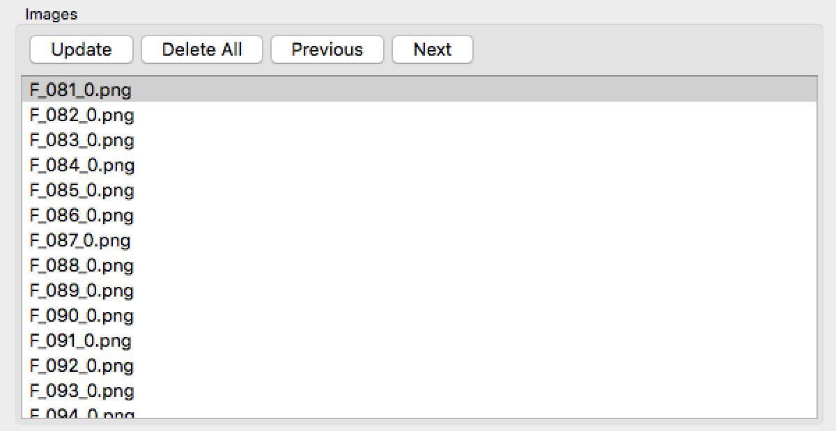
When you start a capture sequence the software clear the list of images shown in the "Images" group, and adds the name of the last file created as a line to the list after the corresponding image is created and the file is stored. The file names are created with the template "F_nF,nI.png" where nF is the frame number as specified by the frame counter, and nI is the image number within this frame.

After the capture sequence completes, or the "STOP" button is pressed, only the names of files created during the last capture session are still displayed in the list. If you now press the "Update" button, the list is updated with the names of all the image files existing in the work directory. If you press the "Delete All" button, all the image files in the work directory will be deleted without warning. If you click the mouse on an element of the list, the corresponding image will be loaded from the file and displayed on the leftmost window. You can use the keyboard "Up" and "Down" keys to navigate the list. Pressing the "Previous" and the "Next" buttons in the "Images" group will produce the same effect.

Camera Calibration

The first step in the calibration process is camera calibration. This is a critical step, and needs to be performed as accurately as possible. You will use the software to automate the image capture process, but you will use the Matlab Camera Calibration Toolkit, as in assignment 2, to perform the camera calibration outside of the software. Then you will load the intrisic camera calibration parameters from the "Calib_Results.mat" file generated by the Matlab Camera Calibration Toolkit.

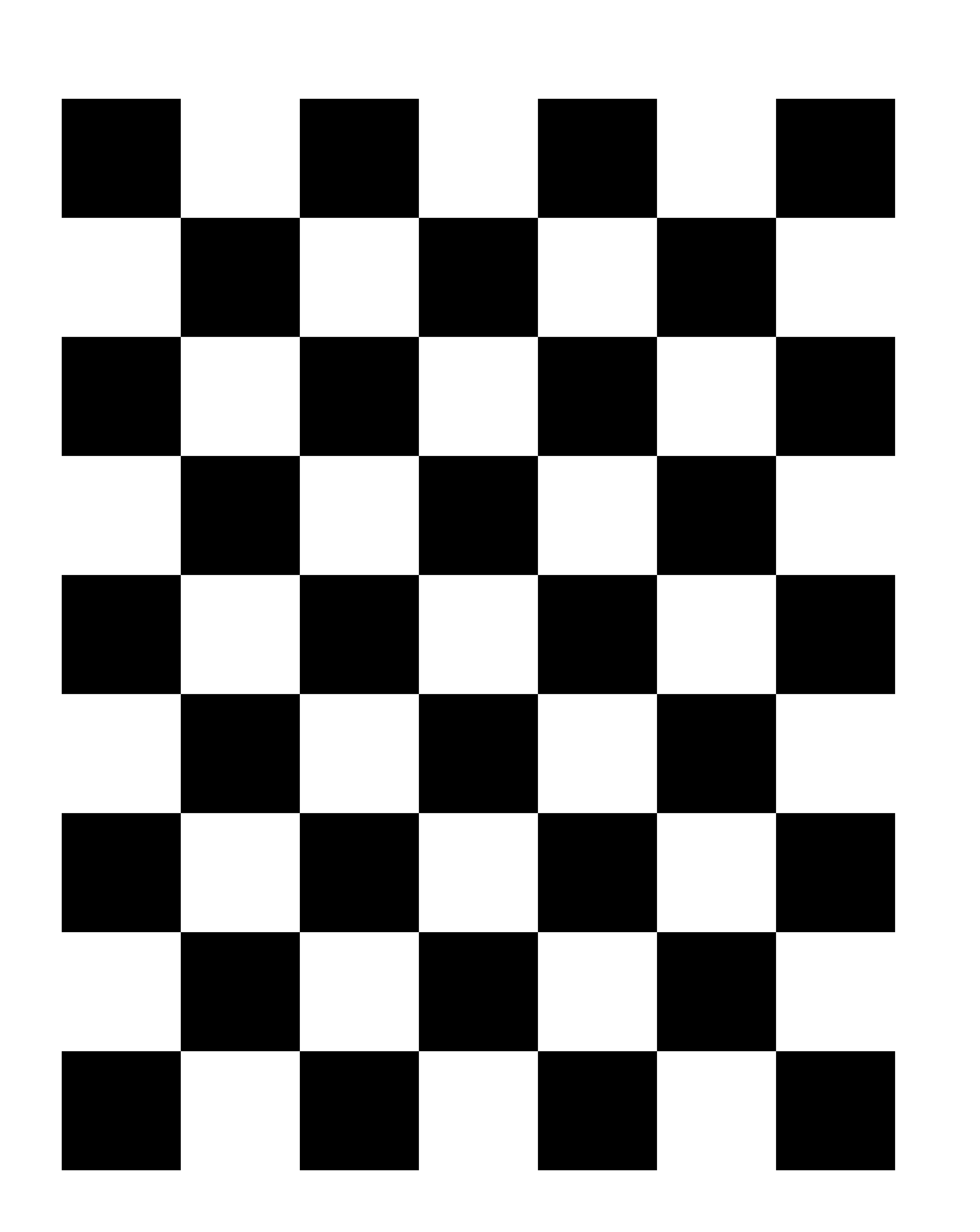
You will need a checkerboard panel of the proper size to perform this step. Download the file named checkerboard-7x9.pdf and print it scaled down so that the resulting print firts within the field of view of the camera within the bounds of the turntable. Keep in mind that the turntable diameter is approximately 160mm, and the maximum height of the object to be scanned should not exceed 160mm. If the object is taller it would not feet in the field of view of the camera. Attach the scaled down checkerboard to a flat hard surface such as a piece of acrylic, aluminum, MDF, plywood, or foam board. I built my camera calibration checkerboard using 1/4 inch MDF board, which is a homogeneous engineered material which is quite flat, and does not deform much over time, or as function of weather conditions. Plywood or foam board may deform over time as function of humidity. Acrylic can be a good choice as well. Use a glue stick or some other liquid adhesive to attach the print to the board, and make sure that there are no bubbles. Using scotch tape to attach the print to the board is not a good idea. The resulting checkerboard board should be as flat as possible. Finally, measure the dimensions of the squares. The two dimensions may be slightly different, as a function of the printer design. Do not measure a single scuare. Measure a number of squares in a row, from end to end, and divide by the number of squares in the row. Repeat for a column. If you measure with a ruler, this process will result in more precise measurements.

Select the camera calibration work directory, where you will save the camera calibration images, and delete all the contents, if the directory is not already empty. In my case this directory would be "/Users/taubin/Teaching/3DP/2016/data/laser-scans/calib/camera". In the "Capture" group, specify the two laser to be off. However, read the Laser Plane Calibration section before you start performing this task, since capturing these images either with one laser in "ON" mode, or both in "CYCLE" mode you could use the same images to perform camera calibration and laser plane calibration. You will use the camera capture automation functionality described above to capture the images, even though to perform camera Set the "Count" parameter to the desired number of images. and press the "START" button. To perform camera calibration you do not necessarily have to use the the turntable. The turntable will turn during the capture sequence, but you can hold the checkerboard in your hand so that it is fully visible within the field of view of the camera while the capture automation process continues. If instead you want to capture one image at a time, set the "Count" value to 1 and uncheck the "Reset Counter" checkbox, so that the next image does not overwrite the last image. You can also add images of the checkerboard placed on the turntable and rotating under the software control. You will have to design and build a checkerboard stand so that the checkerboard board can be placed on the turntable. I build my camera calibration checkerboard attached to a small camera ball mount, with the camera ball mount mounted on top of a heavy base. Ib this way I can change the orientation of the checkerboard, as well as its position on the turntable. Results will be more accurate if the checkerboard is not hold in your hand, but you have to make sure that you have enough images and orientations to cover all the desired work volume. Otherwise large error will result in areas not covered by calibration images.

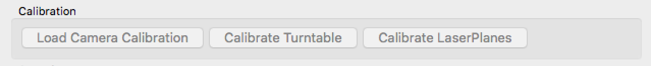
Once you finish capturing the camera calibration images, perform the camera calibration precedure in Matlab using the Matlab Camera Calibration Toolbox. Check the reprojection errors to make sure that your calibration is good. You can delete some bad images if necessary, and recalibrate. You can also add more images to improve the result. Once you are satisfied with the camera calibration that you obtain store the "Camera_Calib.mat" file in the same work directory where you have saved the camera calibration images. Once the software detects the presence of the "Camera_Calib.mat" file in the work directory, the "Load Camera Calibration" button is enabled in the calibration group. Press the "Load Camera Calibration" button to load the data stored in the "Camera_Calib.mat" file. If you replace the "Camera_Calib.mat" file, it will not be loaded automatically.

Turntable Calibration

You will use the results of assignment 3 to calibrate the turntable, i.e. to estimate the turntable plane, the turntable axis of rotation, and the object coordinate system attached to the turntable so that the origin of the coordinate system is located at the intersection of the axis of rotation and the turntable plane, the first two coordinate axes span the turntable plane, and the third coordinate axis spans the axis of rotation.

Select the turntable calibration work directory, where you will save the turntable calibration images, and delete all the contents, if the directory is not already empty. Copy the "Calib_Results.mat" file from the camera calibration work directory into this directory. In my case this directory would be "/Users/taubin/Teaching/3DP/2016/data/laser-scans/calib/turntable".

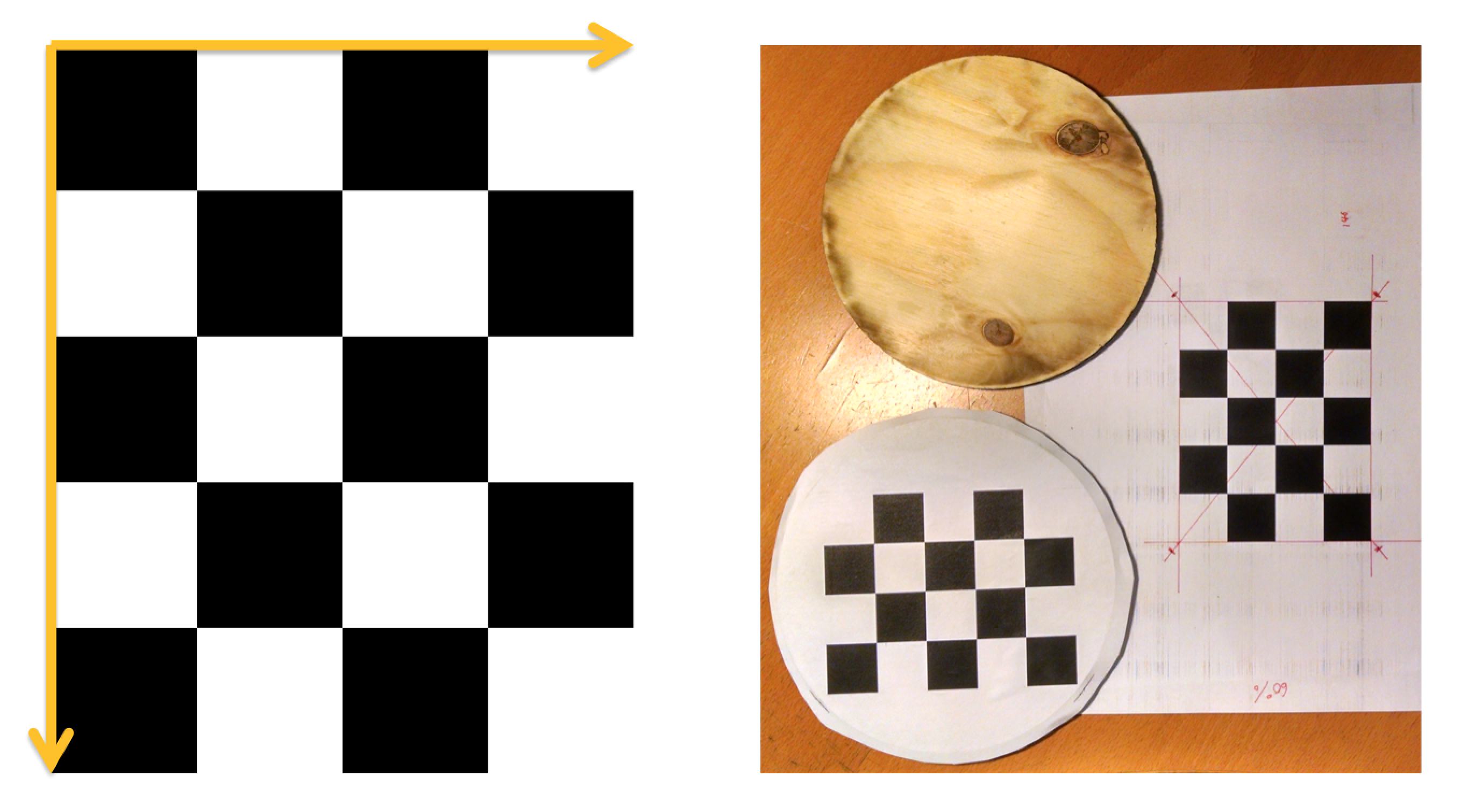
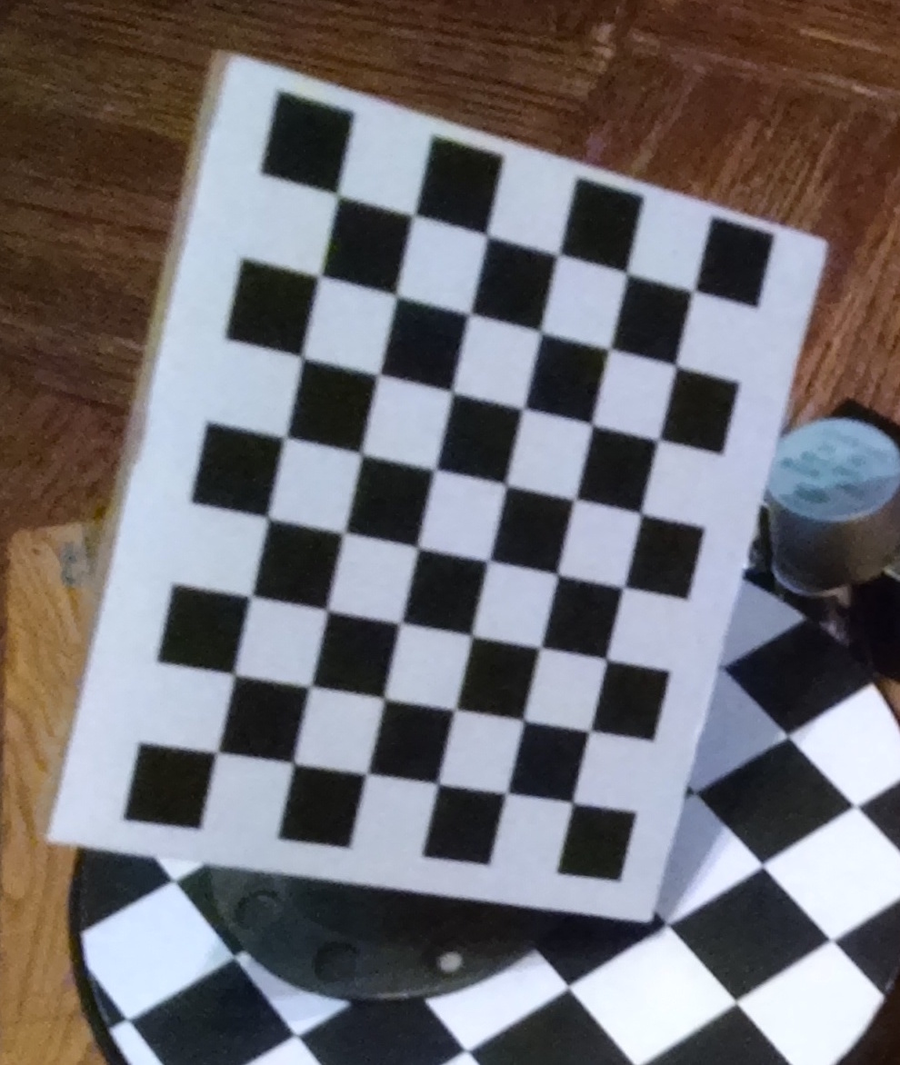
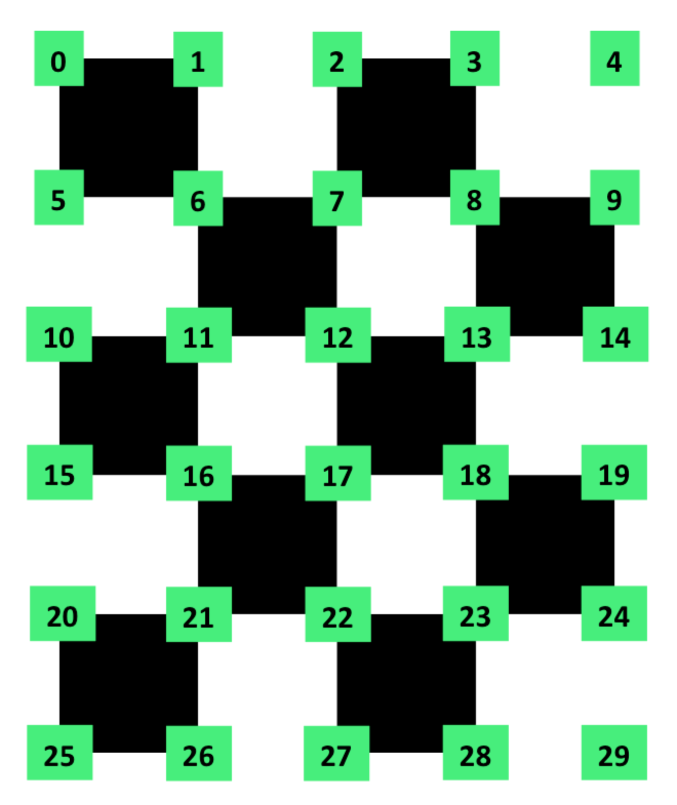
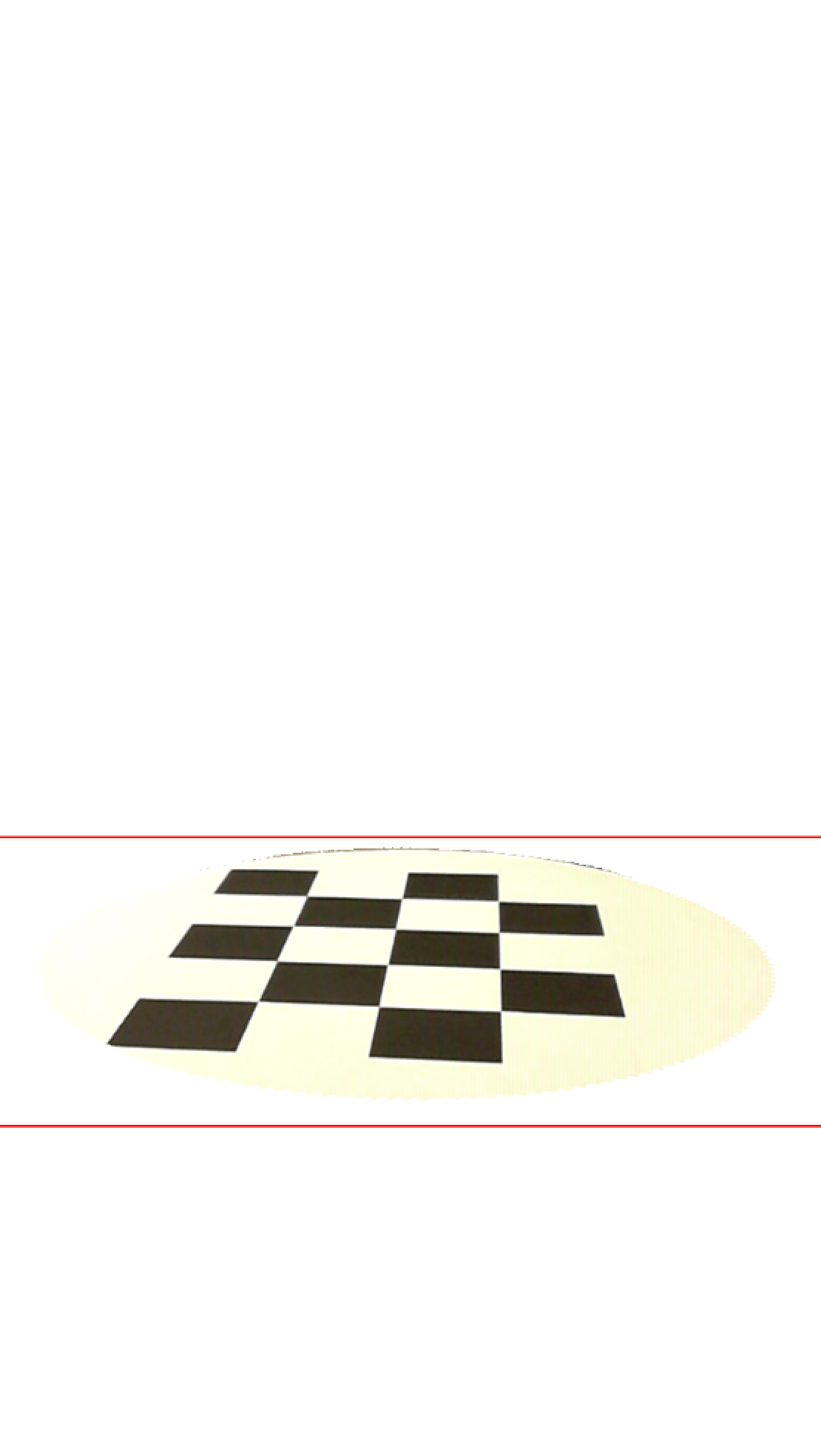
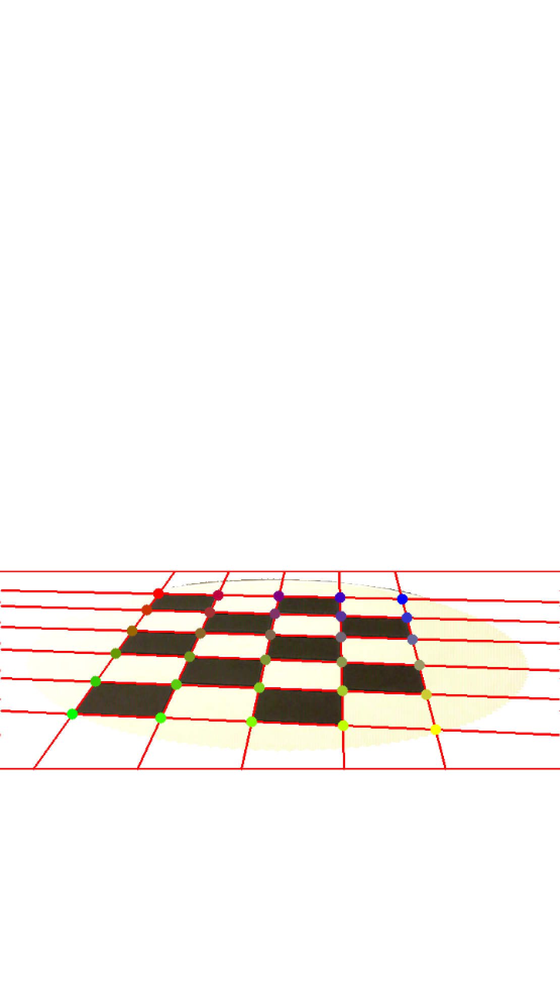
You also need a checkerboard to perform this step, but this one has to be attached to the turntable plane. Because of the small number of pixels covering the checkerboard in the image plane and the severe tilt with respect to the camera, a checkerboard with fewer squares must be used. Otherwise it becomes extremely difficult to detect it. Also, to be able to determine the correspondence between checkerboard corners and detected corners in the image without ambiguity, one of the dimensions of the checkerboard should be even, and the other should be odd. We have determined that a checkerboard with 4 colums and 5 rows works reliably in this case. In such checkerboard only one of the 4 extreme corners is the corner of a black square with an incident x axis of length 4 and y axis of length 5. The following figure shows the chosen checkerboard indices; a checkerboard printed to the proper scale, glued to a turntable top, and trimmed using an X-Acto knife; and an image of the turntable captured by the scanner camera.

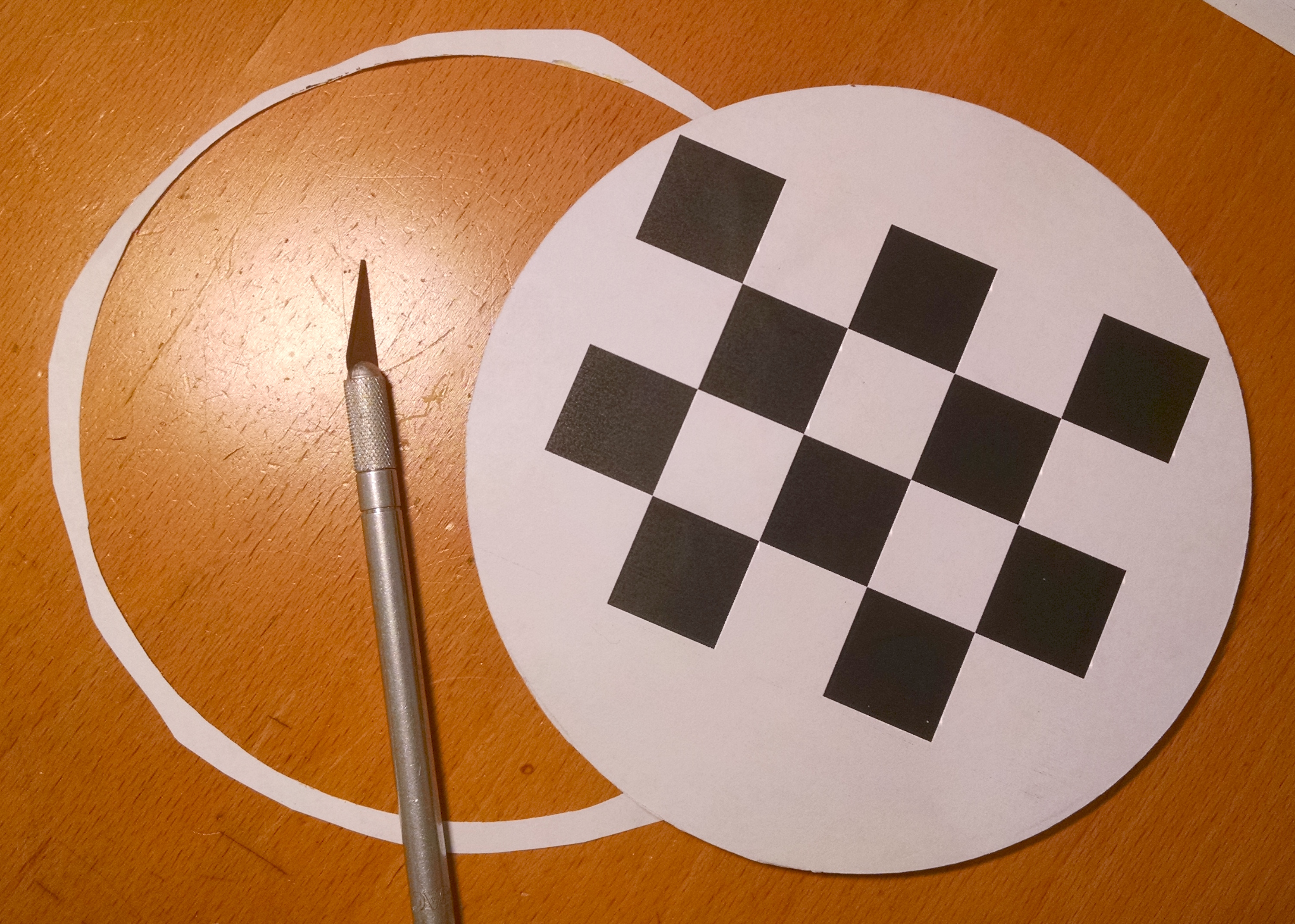
The turntable is designed so that the top surface can be removed. We have laser cut plywood disks that fit the space allocated to the top. Download the file checkerboard-5x4.pdf, print it at the proper scale, and attach it to one of these disks. The disks are approximately 154mm in diameter, but the diameter needs to be adjusted so that they fit tightly. They should not be allowed to move. The checkerboard does not have to be perfectly centered on the disk. The camera intrinsic parameters are already calibrated, and we know that 4 coplanar points are sufficient to estimate the relative pose of the camera with respect to the plane. In our case we are detecting 30 checkerboard corners.

We have developed a checkerboard detection algorithm which requires a mask, and the software includes a method to compute an appropriate mask. The mask is managed in the "Mask" group of the user interface. When you press the "Mask" button, the software will either try to read the mask from a file, or it will try to recompute it as a function of the images present in the turntable calibration work directory. The mask file should be named "mask.png" and should be located in a subdirectory named "tmp" of the turntable calibration work directory. When the software computes a mask, it saves it to this location. When the software tries to read the mask from a file, it reads it from this location. In my case the absolute path of the mask file would be "/Users/taubin/Teaching/3DP/2016/data/laser-scans/calib/turntable/tmp/mask.png". You can create the mask file yourself using an image editing program such as Adobe Photoshop. The image should be of the same dimension as those saved by the software in the work directory, i.e, 720x1280 pixels. The mask is read from the red channel of this image, and the other channels are ignored. The value of the red channel for the pixels on the turntable plane should be equal to 0xff (255), and it should be equal to 0x00 (0) for all the other pixels. Even though the green and blue channels are ignored, when the software creates the mask image it assigns the value 0x00 (0) to all the pixels in the green and blue channels. To create your own mask using an image editor, capture one image with the software, and use the corresponding image saved in the turntable calibration work directory as a starting point. Since the black squares do not touch the disk boundary, the mask can be eroded a couple of pixels as a margin of safety. If the disk is not perfectly planar, the masking may not be perfect, and artifacts may result near the disk boundary in some locations.

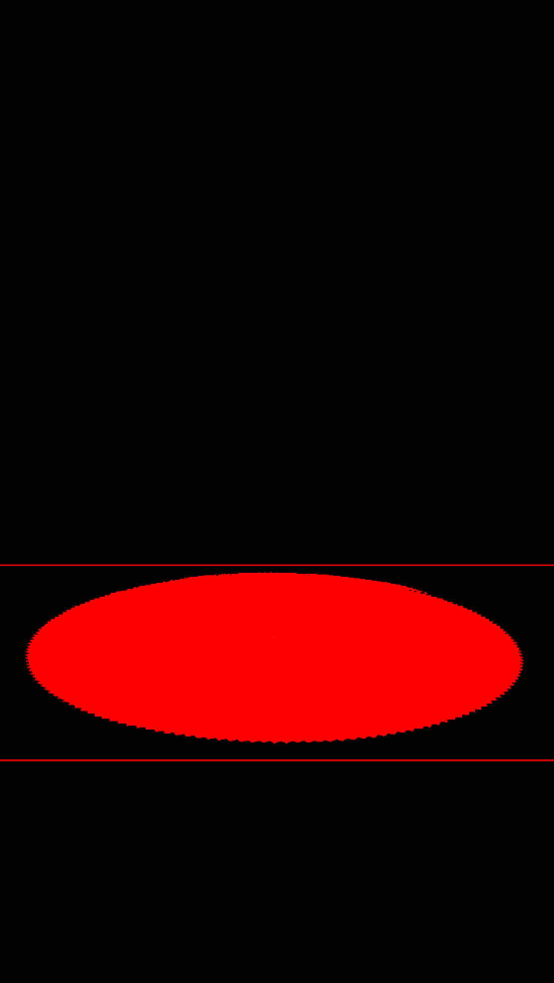
If the mask file is not present, or if the "Recompute" checkbox is checked, the software will try to compute a mask as a function of the images currently stored in the turntable calibration work directory. For this process to result in a valid mask, you should first delete all the images by pressing the "Delete All" button in the Image group, and then capture a new sequence where the turntable undergoes a full rotation. With the deafult turntable parameters a full rotation requires 180 frames. In the "Capture" group set the "Count" value to 180, specify the two lasers to be off, and check the "Reset Counter" checkbox. Then press the "START" button, and wait until the process finishes. The same sequence will be used after the mask is computed to detect the checkerboards and to perform the turntable calibration. Make sure that the illumination does not change at all during the capture process, and also that, except for the rotation of the turntable, no other scene changes occur. The pixels values for the pixels not corresponding to points on the turntable plane should not change during the capture process.

The "Min" and "Max" buttons remain in the user interface only for illustration purposes, since the mask is computed as a function of the two images produced when these buttons are pressed. So is the "Threshold" checkbox. For proper computation of the mask it should be checked. The actual mask image is the result of thresholding the image produced when the "Threshold" checkbox is not checked. The "Modulate" checkbox determines how the captured images are displayed after a mask has been read or computed. The second picture in the previous figure shows a captured image displayed modulated by the mask. The current checkerboard detection algorithm operates correctly only on these masked images. The third picture in the previous image shows the result of applying the checkerboard detection algorithm to the second picture.

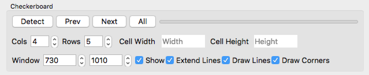
The "Checkerboard" group controls the behavior of the checkerboard detection algorithm. The "Detect" button runs the checkerboard detection algorithm on the image currently on display. This image must have the mask applied to it for the algorithm to be successful. The "Previous" button first selects the previous image in the image list, and then it applies the checkerboard detection algorithm to it. The "Next" button performs the same function in the opposite direction. By pressing the "Next" button for each captured image, the checkerboard detection algorithm is applied to all the images. The checkerboard detection algorithm always returns a list of line segments, which are subsequently rendered on the masked image. If successful, these line segments should correspond to the boundaries of checkerboard squares. If not successful some segments may be missing, and/or some additional segemnts may be present. If the checkerboard detection algorithm fails on a particular image, you should delete that image from the turntable calibration work directory before you perform the turntable calibration step. The "All" button runs the checkerboard detection algorithm on all the images.

The number of rows and columns of the checkerboard attached to the turntable plane are specified in the "Cols" and "Rows" fields. If the checkerboard detection algorithm detects exactly (cols+1)+(rows+1) lines in the image, then it returns the 2D coordinates of the (cols+1)*(rows+1) checkerboard corners in row scan order at subpixel resolution. If it does not detect the (cols+1)+(rows+1) lines, it does not compute coordinates and it returns an error message.

You should enter the dimensions of the checkerboard cells in the "Cell Width" and "Cell Height" fields. Once these values are defined, and the checkerboard detection algorithm has been run successfully on all the images, the "Calibrate Turntable" button in the "Calibrate" group is enabled. Once it is enabled, you can press the "Calibrate" button to estimate to estimate the turntable plane, the turntable axis of rotation, and the object coordinate system attached to the turntable so that the origin of the coordinate system is located at the intersection of the axis of rotation and the turntable plane, the first two coordinate axes span the turntable plane, and the third coordinate axis spans the axis of rotation. Once the turntable is calibrated, the 3D View camera model will be updated to display a view of the 3D scen from a point of view similar to the camera's.

Laser Plane Calibration

You will use the results of assignment 3 to perform laser plane calibration. To calibrate the laser planes you need to capture images of checkerboards illuminated by the lasers. As explained in the Camera Calibration section, with one laser on, or with both lasers cycling, the same images can be used both to perform camera calibration, and laser plane calibration. This is so because, in addition to the camera intrinsic parameters, the "Camera_Calib.mat" file produced by the Matlab Camera Calibration Toolbox also contains estimated extrinsic parameters for each of the images used in the calibration process.

Select the laser plane calibration work directory, and make sure that it is empty. If you decide to use the same images for camera and laser plane calibration, copy the "Camera_Calib.mat" file into this directory and rename it "Laser_Calib.mat". Otherwise, capture a new sequence with one laser on or with the two lasers cycling, run camera calibration again using the Matlab Camera Calibration Toolbox, and rename the resulting "Camera_Calib.mat" file as "Laser_Calib.mat".

Once The "Laser_Calib.mat" file exists in the work directory, the "Calibrate Laser Planes" button is enabled. When you press this button, the "Laser_Calib.mat" file isloaded, and then you need to detect the illuminated points in each of the images, and then estimate the equations of the planes. Whether only one or two planes are estimated depends on the laser settings in the "Capture" group.

3D Scanning

Finally, you are ready to start 3D scanning objects. Once the camera is calibrated, the turntable is calibrated, and at least one laser plane is calibrated, the "SCAN" button in the "3D Scanning" group is enabled. To scan an object, first select a new work directory, and make sure that it is empty. Place the object to be scanned on the turntable. In the "Capture" group, set the capture parameters. One of the lasers can be in "OFF" mode, but at least one of the lasers should be in "CYCLE" mode. None of the lasers should be in "ON" mode.

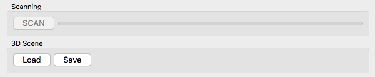
Once you press the "SCAN" button the software will run as when you press an image capture sequence, but after each frame is completed it will call your laser detection and triangulation methods to generate additional points. If only one laser is in "CYCLE" mode, the methods will be called once per frame. If both lasers are in "CYCLE" mode, then the methods will be called twice per frame. The laser detection method will be called with two images as arguments; one image where both lasers are off, and a second image where one laser is on. You should implement a laser detection algorithm more robust that the one that you have implemented before using the two images.

Tasks

In addition to all the tasks defined above, you will have to implement the following methods, which are called by the software. To calibrate the turntable you need to implement the following method, which takes as inputs the camera calibration intrinsic parameters, and for each turntable checkerboard image a vector of 2D checkerboard coordinates (because z=0), and a second vector of 2D image coordinates produced by the checkerboard detection algorithm. It produces as output the 2D coordinates of the center of rotation in checkerboard coordinates, and the world coordiante system, where the first two axes of the rotation matrix spans the turntable plane, the third axis spans the axis of rotation, and the translation vector describes the center of rotation in camera coordinates.

  void calibrateTurntable
  ( // inputs
   Matrix3d const&                    K,
   Vector5d const&                    kc,
   QVector<QVector<Vector2d> > const& worldCoord,
   QVector<QVector<Vector2d> > const& imageCoord,
   // outputs
   Vector2d&                          centerCoord,
   Matrix3d&                          worldRotation,
   Vector3d&                          worldTranslation);

You also need to implement a new method to calibrate the laser plane. This method takes as inputs the camera intrinsic parameters, a number of images of checkerboards illuminated by one laser, for each image a rotation and translation, and produces as output the implicit equation of the laser plane. The images are those used to generate the "Laser_Calib.mat" file using the Matlab Camera Calibration Toolbox. The intrinsic parameters, as well as the rotations and translations are those read from that file. You will have to use the first laser line detection algorithm that you developed for a single image.

  void calibrateLaserPlane
  ( // inputs
   Matrix3d const&          K,
   Vector5d const&          kc,
   QVector<QString>  const& laserImageFileName,
   QVector<Matrix3d> const& R,
   QVector<Vector3d> const& T,
   // outputs
   Vector4d&                laserPlane);
 

Finally, you will have to implement a method to generate 3D point from each image capture while scanning an object. This method takes as input the camera intrinsic parameters, the world coordinate system produced by your calibrateTurntable() method, the angle of rotation, one background image with the lasers off, one foreground image with one laser one, and the implicit equation of the laser plane. It should produce a vector of 3D coordinates of triangulated cpoints, which the software will insert in the 3D scene graph to be displayed in the 3D View. This method will be called after the capture of each frame

  void scan
  ( // inputs
   Matrix3d const&    K,
   Vector5d const&    kc,
   Matrix3d const&    worldRotation,
   Vector3d const&    worldTranslation,
   float const        angle,
   QImage const &     backgroundImage,
   QImage const &     foregroundImage,
   Vector4d const&    laserPlane,
   // outputs
   QVector<Vector3d>& worldCoord);

3   Submission Instructions

You must upload a Zip file of the complete application, including your implementation of the required functions, in canvas. If you need to communicate with the TA some implementation details, issues, exceptional results, extra work done, or anything else that you want to be considered while grading, do it so by writing a comment in the 'homework4.cpp' file, or add a document in the root folder of the software.

You must also include a folder called 'results' with screen shots of the application showing the reconstructed points, as well as the reconstructed point clouds resulting from pressing the "Save" button ine the "3D Scene" group.