Camera Calibration
The Ideal Pinhole Camera Model
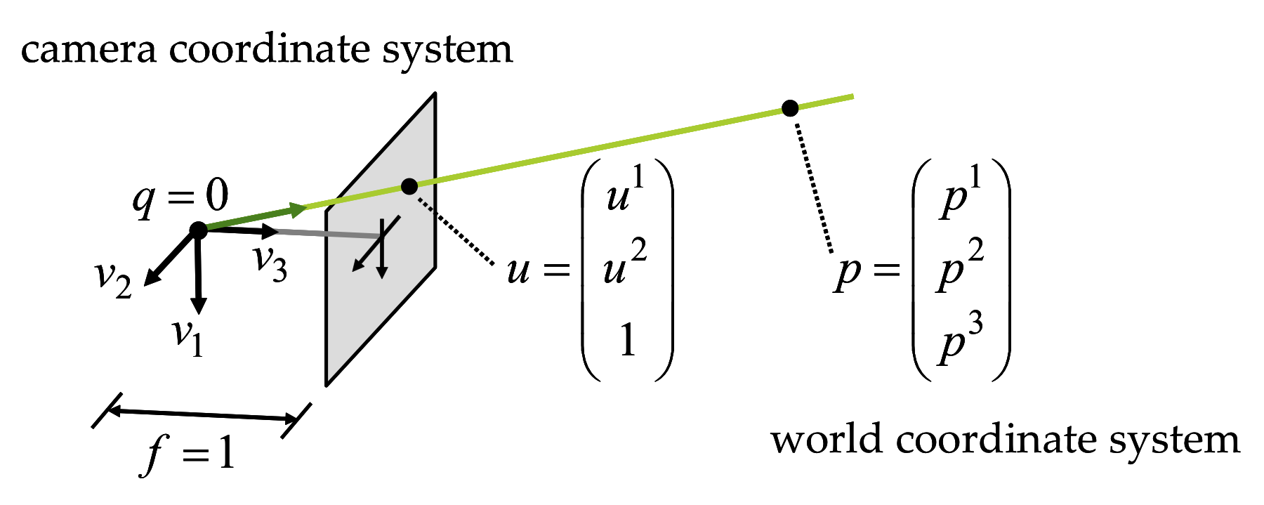
Figure 1 The ideal pinhole camera.
In the ideal pinhole camera shown in Figure 1, the center of projection \(q\) is at the origin of the Canonical Camera Coordinate System, the vectors \(v_1\) \(v_2\) and \(v_3\) form an orthonormal basis, the image plane is spanned by the vectors \(v_1,v_2\), and it is located at distance \(f=1\) from the origin \[\{ u^1v_1+u^2v_2+q : u^1,u^2\in\mathbb{R}\}\] An arbitrary 3D point \(p^1v_1+p^2v_2+p^3v_3+q\) with coordinates \(p=(p^1,p^2,p^3)^t\) belongs to this plane if \(p^3=0\), otherwise it projects onto an image point with the following image coordinates \begin{equation} \left\{ \begin{matrix} u^1 & = & p^1/p^3\cr u^2 & = & p^2/p^3 \end{matrix} \right. \label{eq:perspective-projection} \end{equation} The projection of a 3D point \(p\) with coordinates \((p^1,p^2,p^3)^t\) has homogeneous image coordinates \(u=(u^1,u^2,1)\) if for some scalar \(\lambda\neq 0\), we can write \begin{equation} \lambda\; \left( \begin{matrix} u^1\cr u^2\cr 1 \end{matrix} \right) = \left( \begin{matrix} p^1\cr p^2\cr p^3 \end{matrix} \right)\;. \label{eq:ideal-pinhole-projection} \end{equation} Note that not every 3D point has a projection on the image plane. Points without a projection are contained in a plane parallel to the image passing through the center of projection.
The General Pinhole Camera Model
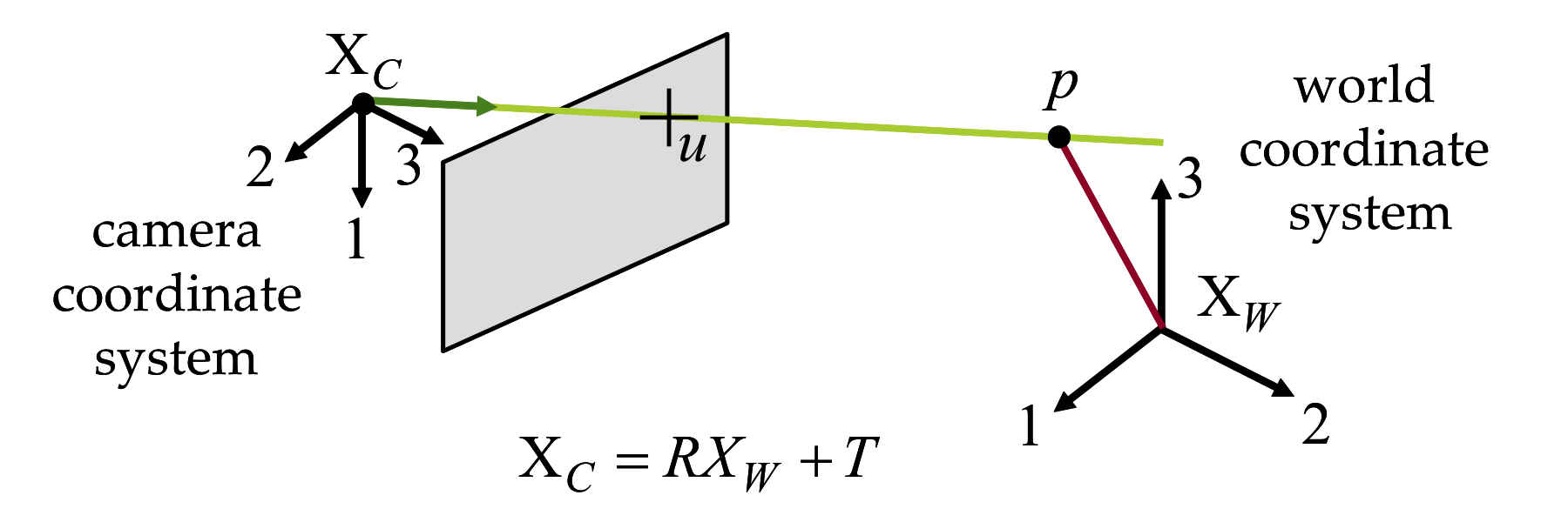
Figure 2 The general pinhole model.
The center of a general pinhole camera is not necessarily placed at the origin of the world coordinate system and may be arbitrarily oriented. However, it does have a camera coordinate system attached to the camera, in addition to the world coordinate system (see Figure 2). A 3D point \(p\) has world coordinates described by the vector \(p_W=(p_W^1,p_W^2,p_W^3)^t\) and camera coordinates described by the vector \(p_C=(p_C^1,p_C^2,p_C^3)^t\). These two vectors are related by a rigid body transformation specified by a translation vector \(t\in\mathbb{R}^3\) and a rotation matrix \(R\in\mathbb{R}^{3\times 3}\), such that \[ p_C=R\,p_W+t\;. \] In camera coordinates, the relation between the 3D point coordinates and the 2D image coordinates of the projection is described by the ideal pinhole camera projection of Equation \ref{eq:ideal-pinhole-projection}, with \(\lambda u = p_C\). In world coordinates this relation becomes \begin{equation} \lambda\,u = R\,p+t= p^1r_1+p^2r_2+p^3r_3+t\;. \label{eq:general-pinhole-projection} \end{equation} where \(p=p_W\) are the world coordinates of the 3D point, and \(r_1,r_2\) and \(r_3\) are the three column vectors of the rotation matrix \(R=[r_1,r_2,r_3]\), which form an orthonormal basis. The parameters \((R,t)\), which are referred to as the extrinsic parameters of the camera, describe the location and orientation of the camera with respect to the world coordinate system, and comprise six degrees of freedom.
Equation \ref{eq:general-pinhole-projection} assumes that the unit of measurement of lengths on the image plane is the same as for world coordinates, that the distance from the center of projection to the image plane is equal to one unit of length, and that the origin of the image coordinate system has image coordinates \(u^1=0\) and \(u^2=0\). None of these assumptions hold in practice. For example, lengths on the image plane are measured in pixel units, while they are measured in meters or inches for world coordinates, the distance from the center of projection to the image plane can be arbitrary, and the origin of the image coordinates is usually on the upper left corner of the image. In addition, the image plane may be tilted with respect to the ideal image plane. To compensate for these limitations of the current model, a matrix \(K\in\mathbb{R}^{3\times 3}\) is introduced in the projection equations to describe intrinsic parameters as follows. \begin{equation} \lambda\,u = K(R\,p\,+\,t) \label{eq:general-pinhole-projection-with-intrinsic} \end{equation} The matrix \(K\) has the following form \[ K= \left( \begin{matrix} f\,s_1 & f\,s_\theta & o^1 \cr 0 & f\,s_2 & o^2 \cr 0 & 0 & 1 \end{matrix} \right)\;, \] where \(f\) is the focal length (i.e., the distance between the center of projection and the image plane). The parameters \(s_1\) and \(s_2\) are the first and second coordinate scale parameters, respectively. Note that such scale parameters are required since some cameras have non-square pixels. The parameter \(s_\theta\) is used to compensate for a tilted image plane. Finally, \((o^1,o^2)^t\) are the image coordinates of the intersection of the vertical line in camera coordinates with the image plane. This point is called the image center or principal point. Note that all intrinsic parameters embodied in \(K\) are independent of the camera pose. They describe physical properties related to the mechanical and optical design of the camera. Since in general they do not change, the matrix \(K\) can be estimated once through a calibration procedure and stored (as will be described in the following chapter). Afterwards, image plane measurements in pixel units can immediately be normalized, by multiplying the measured image coordinate vector by \(K^{-1}\), so that the relation between a 3D point in world coordinates and 2D image coordinates is described by Equation \ref{eq:general-pinhole-projection}.
Modeling Lens Distortion
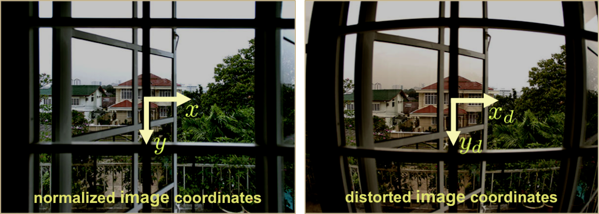
Figure 2 Non-linear Lens Distortion.
Real cameras also display non-linear lens distortion, which is also considered intrinsic. Lens distortion compensation must be performed prior to the normalization described above. The camera matrix \(K\) does not account for lens distortion because the ideal pinhole camera does not have a lens. To more accurately represent a real camera, radial and tangencial lens distortion parametes should be added to the camera models.
Radial Lens Distortion
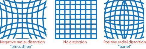
Figure 3 Radial Lens Distortion.
Tangencial Lens Distortion
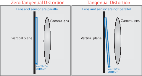
Figure 4 Tangential Lens Distortion.
Tangential distortion occurs when the lens and the image plane are not parallel. The tangential distortion coefficients model this type of distortion. A complete lens distortion model is obtained by adding tangencial distortion coefficients \(\tau_1\) and \(\tau_2\) to the radial distortion model of equation \ref{eq:radial-distortion} \begin{equation} \left(\begin{matrix} x_d \\ y_d \end{matrix}\right) = \Phi \left(\begin{matrix} x_u \\ y_u \end{matrix}\right) \label{eq:radial-tagential-distortion-mapping} \end{equation} where \(\Phi\) is the \(2D\rightarrow 2D\) polynomial mapping \begin{equation} \Phi \left(\begin{matrix} x_u \\ y_u \end{matrix}\right) = \left(\begin{matrix} x_d\,(1 + k_1 r^2 + k_2 r^4 + k_3 r^6) + 2 \tau_1 x_d y_d + \tau_2 (r^2 + 2 x_d^2) \\ y_d\,(1 + k_1 r^2 + k_2 r^4 + k_3 r^6) + \tau_1 (r^2 + 2 y_d^2) + 2 \tau_2 x_d y_d \end{matrix}\right) \label{eq:radial-tagential-distortion} \end{equation} To undistort a distorted image, the inverse mapping \(\Phi^{-1}\) has to be evaluated, but no closed-form expression for this inverse mapping exists. In practice, the evaluation is performed through a look-up table process.
Overall, this camera model with lens distortion comprises up to eleven intrinsic parameters \begin{equation} \Lambda = \{f, s_x, s_y, s_\theta, c_x, c_y, k_1, k_2, k_3, \tau_1, \tau_2\} \label{eq:intrinsic-parameters} \end{equation} in addition to the extrinsic parameters, or pose, with six degrees of freedom, described by the rotation matrix \(R=[r_1 r_2 r_3]\) and translation vector \(t\).
Geometric Camera Calibration
Geometric Camera Calibration refers to procedures to estimate the camera model parameters as described above. These parameters are used to correct for lens distortion, measure the size of an object in world units, and to determine the location of the camera in the scene. Camera Calibration is a required step for all 3D scanning algorithms. Camera parameters include intrinsics, extrinsics, and distortion coefficients. To estimate the camera parameters, we need to have 3D world points and their corresponding 2D image points. We can get these correspondences using multiple images of a calibration pattern, such as a checkerboard. Using the correspondences, we can solve for the camera parameters. After the camera is calibrated, to evaluate the accuracy of the estimated parameters, we can plot in 3D the relative locations of the camera and the calibration pattern, calculate the reprojection errors, and calculate the parameter estimation errors.Mathematics of Camera Calibration
The Mathematics of Camera Calibration with a 3D rig and with planar patterns is described, for example, in Ma, Soatto, Kosecka, and Sastry, An Invitation to 3-D Vision: From Images to Geometric Models, Springer Verlag, 2003. Section [6.5 Calibration with Scene Knowledge] (6.5.2 Calibration With A Rig; 6.5.3 Calibration with a Planar Pattern).
Camera Calibration Methods
Camera calibration requires estimating the parameters of the general pinhole model described above. At a basic level, camera calibration requires recording a sequence of images of a calibration object, composed of a unique set of distinguishable features with known 3D displacements. Thus, each image of the calibration object provides a set of 2D-to-3D correspondences, mapping image coordinates to scene points. Naively, one would simply need to optimize over the set of 11 intrinsic camera model parameters so that the set of 2D-to-3D correspondences are correctly predicted (i.e., the projection of each known 3D model feature is close to its measured image coordinates).
Many methods have been proposed over the years to solve for the camera parameters given such correspondences. In particular, the factorized approach originally proposed Zhang [Zha00] is widely-adopted in most community-developed tools. In this method, a planar checkerboard pattern is observed in two or more orientations (see Figure 5). From this sequence, the intrinsic parameters can be estimated. Afterwards, a single view of a checkerboard can be used to estimate the extrinsic parameters. Given the relative ease of printing 2D patterns, this method is commonly used in computer graphics and vision publications.
Recommended Calibration Software
A comprehensive list of calibration software is maintained by Bouguet on the Camera Calibration Toolbox website. An alternative camera calibration package is the Matlab Camera Calibration Toolbox. Otherwise, OpenCV replicates many of its functionalities, while supporting multiple platforms. A CALTag checkerboard and software is yet another alternative. CALTag patterns are designed to provide features even if some checkerboard regions are occluded.
Matlab Camera Calibration Toolbox
In this section we describe, step-by-step, how to calibrate your camera using the Camera Calibration Toolbox for Matlab. We also recommend reviewing the detailed documentation and examples provided on the toolbox website. Specifically, new users should work through the first calibration example and familiarize themselves with the description of model parameters (which differ slightly from the notation used in these notes).
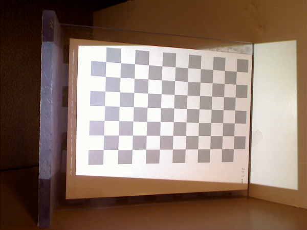
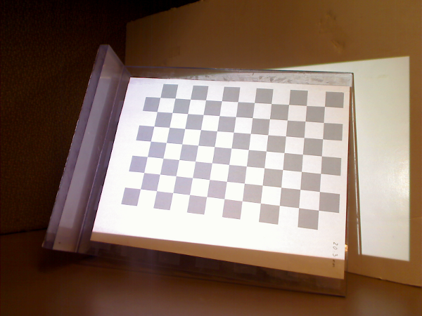
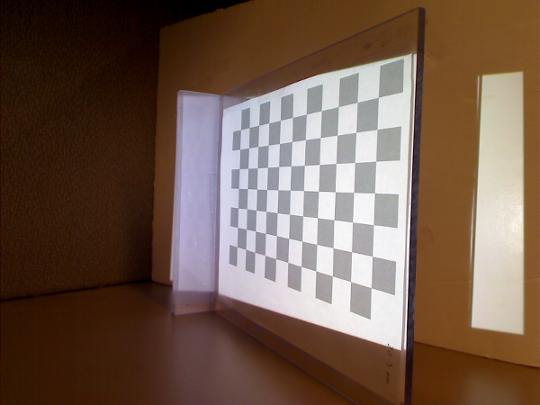
Figure 5 Camera calibration images containing a checkerboard with different orientations throughout the scene.
Begin by installing the toolbox, available for download at the Caltech Camera Calibration software website. Next, construct a checkerboard target. Note that the toolbox comes with a sample checkerboard image; print this image and affix it to a rigid object, such as piece of cardboard or textbook cover. Record a series of 10--20 images of the checkerboard, varying its position and pose between exposures. Try to collect images where the checkerboard is visible throughout the image, and specially, the checkerboard must cover a large region in each image.
Using the toolbox is relatively straightforward. Begin by adding the toolbox to your Matlab path by selecting \(\textsf{File} \rightarrow \textsf{Set Path...}\). Next, change the current working directory to one containing your calibration images (or one of our test sequences). Type \(\texttt{calib}\) at the Matlab prompt to start. Since we are only using a few images, select \(\textsf{Standard (all the images are stored in memory)}\) when prompted. To load the images, select \(\textsf{Image names}\) and press return, then \(\texttt{j}\) (JPEG images). Now select \(\textsf{Extract grid corners}\), pass through the prompts without entering any options, and then follow the on-screen directions. The default checkerboard has 30mm\(\times\)30mm squares but the actual dimensions vary from printer to printer, you should measure your own checkerboard and use those values instead. Always skip any prompts that appear, unless you are more familiar with the toolbox options. Once you have finished selecting corners, choose \(\textsf{Calibration}\), which will run one pass though the calibration algorithm. Next, choose \(\textsf{Analyze error}\). Left-click on any outliers you observe, then right-click to continue. Repeat the corner selection and calibration steps for any remaining outliers (this is a manually-assisted form of bundle adjustment). Once you have an evenly-distributed set of reprojection errors, select \(\textsf{Recomp. corners}\) and finally \(\textsf{Calibration}\). To save your intrinsic calibration, select \(\textsf{Save}\).
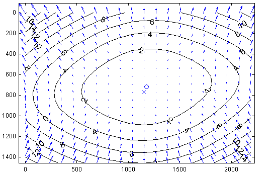
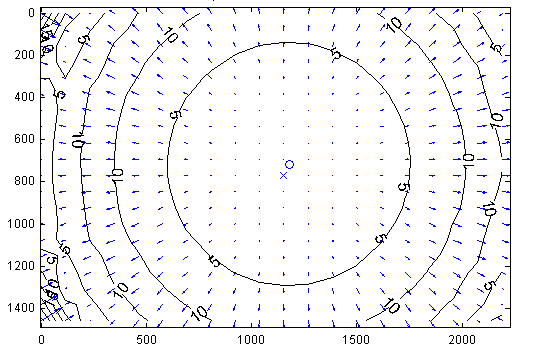
Figure 6 Camera calibration distortion model. (Left) Tangential Component. (Right) Radial Component. Sample distortion model of the Logitech C920 Webcam. The plots show the center of distortion \(\times\) at the principal point, and the amount of distortion in pixel units increasing towards the border.
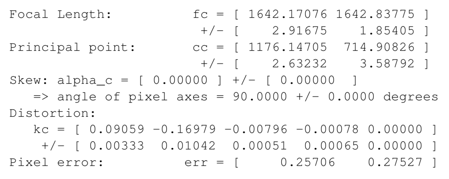
From the previous step you now have an estimate of how pixels can be converted into normalized coordinates (and subsequently optical rays in world coordinates, originating at the camera center). Note that this procedure estimates both the intrinsic and extrinsic parameters, as well as the parameters of a lens distortion model. Typical calibration results, illustrating the lens distortion model is shown in Figure 6. The actual result of the calibration is displayed below as reference.
Logitech C920 Webcam sample Calibration Result
Camera Calibration with OpenCV
OpenCV includes the calib3d module for camera calibration, which we will use in the course software.