
Assignment 2:
Camera calibration and Triangulation
Instructor: Gabriel Taubin
Assignment developed by: Daniel Moreno
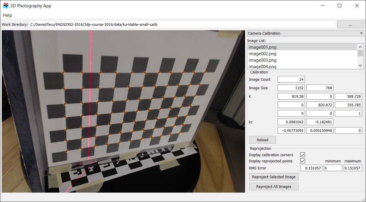
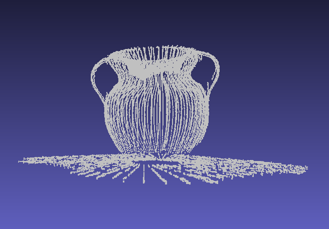
Figure 1: 3D Photography software displaying a calibration image (left) and a pointcloud result of triangulation (right). Click images to zoom in.
Downloads: 3dp-course-2016-assignment2-2.0.zip, Camera-Calibration Toolbox, data-turntable-small.zip, turntable-small-calib.zip
Introduction
In this assignment we will calibrate our camera, validate the calibration by reprojecting a set of corners on the image plane, and implement Ray-Plane triangulation to create a 3D pointcloud.
1 Camera Calibration
Your first task is to calibrate a camera of your choice. Download the Camera Calibration Toolbox for MATLAB. The version in this assignment page works with PNG images, in addition to other supported formats, opposite to the official download.
Unzip the file to some folder (e.g. c:\3dp\TOOLBOX_calib) and add this folder to your MATLAB path, or remember before use to execute a command in MATLAB similar to this:
addpath('c:\3dp\TOOLBOX_calib')
Refer to the Toolbox's webpage to learn how to use it.
Print a copy of the calibration pattern in 'TOOLBOX_calib/calibration_pattern/pattern.pdf', or create your own using MATLAB's 'checkerboard' function. Fix the pattern on a planar surface such as a table or a piece of glass, capture 5 or more images of the pattern in different orientations, and use the toolbox to calibrate your camera. In particular, read carefully and follow the directions of the First calibration example on the toolbox documentation.
To capture calibration images any software may be used, including the 3D Photography software which works with most USB cameras. In the 3D Photography software, switch to the 'Camera Capture' panel, select your camera, and click 'Preview'. Rotate the images if required. Press 'Capture One' button to capture images and number them from 1 to N.
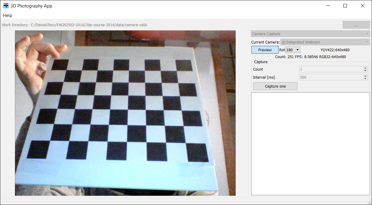
Figure 2: calibration image capture with 3D Photography software.
Load your images in the toolbox and calibrate your camera. You MUST have a reprojection error of less than 0.5 pixels to get full points in this assignment. A sample result is the following:
Focal Length:          fc = [ 641.83006   647.07169 ] +/- [ 3.15740   2.84094 ]
Principal point:       cc = [ 319.70695   270.24005 ] +/- [ 4.38610   3.62526 ]
Skew:             alpha_c = [ 0.00000 ] +/- [ 0.00000  ]
   => angle of pixel axes = 90.00000 +/- 0.00000 degrees
Distortion:            kc = [ -0.02144   0.16541   0.00447   0.00117  0.00000 ]
                        +/- [  0.02930   0.19959   0.00190   0.00266  0.00000 ]
Pixel error:          err = [ 0.16149   0.13555 ]
Save the calibration and take a screenshot of the extrinsic parameter plot, similar to Figure 3 below.
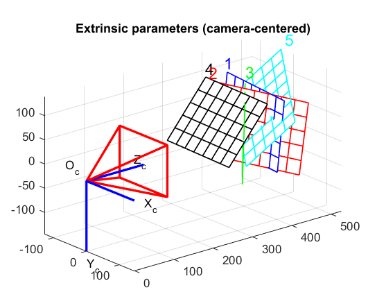
Figure 3: Visualization of the camera extrinsic parameters from the Calibration Toolbox
1.1 Submission
Upload to Canvas a Zip file with your pattern images, the calibration result files 'Calib_Results.m' and 'Calib_Results.mat', and a screenshot of the Extrinsic parameters visualization.
2 Reprojection to images
You second task is to complete the code in the 3D Photography software to reproject the calibration 3D corners back onto 2D image points.
The function 'hw2::reprojectPoints(...)' is found in the file 'homework/homework2.cpp. It receives camera intrisics (K, kc) and extrinsics (R,T) parameters, as well as, the 3D coordinates of the checkerboard coordinates (worlPoints). Your task is to use these parameters to reproject each of the 3D points onto the image plane and save the reprojected 2D points in the output 'reprojectedPoints'. In addition, you must compare your reprojected points with the original 2D image points, given in 'imagePoints', and compute the Root Mean Square Error (RMSE). The RMSE is the return value of this function. double reprojectPoints(Matrix3d const& K, Vector5d const& kc,
Matrix3d const& R, Vector3d const& T,
QVector const& worldPoints,
QVector const& imagePoints,
QVector & reprojectedPoints);
To test your code, switch to the 'Camera Calibration' panel in the software, set the working directory to the calibration folder created in the previous section. This folder must contain the captured images and the file 'Calib_Results.mat'. The software will load this file and display the calibration parameters. Select an image and press 'Reproject Selected Image' to call your reprojection function.

Figure 4: Camera Calibration Panel
During reprojection, each 3D point must be transformed to camera coordinates using the extrinsic parameters, the transformed point is projected to the canonical image plane, and the lens distortion model is used to correct the points. Finally, the intrisic parameters are used to transform the point to image coordinates. Most of these is explained in detail, including equations, in the calibration parameters webpage.
- \(p_c = R*p_w+T\)
- \(p_n = (x/z, y/z) \)
- \(p_d = F(kc, r^2) * p_n \), \(F\) is the lens distortion function.
- \(p_i = K*p_d \)
Use the reprojected points and the original image points to calculate the Root Mean Square Error (RMSE):
$$\text{RMSE} = \sqrt{\frac{1}{2N} \sum_{n=1}^N ||p_n - \hat{p}_n||^2}$$We use the Eigen Library for Matrix and Vector operations. Visit the Quick reference guide for a summary of common operations if you are new to Eigen.
3 Laser line triangulation
In this section, you have to complete the code for 3D point triangulation. Make sure to copy your laser line detection implementation file 'homework1.cpp' from your previous assignment to the new code.
  QVector triangulate(Matrix3d const& K, Vector5d const& kc,
                                Matrix3d const& R, Vector3d const& T,
                                Vector4d const& laserPlane, double turntableAngle,
                                QImage image);
The function 'hw2::triangulate(...)' receives Camera and Turntable calibration as input parameters, together with an image. The function will call 'hw1::detectLaser()' to find a vertical laser line, and it will triangulate using plane-ray intersection each of the pixels on the laser line. The function returns a vector of 3D points. Each image has associated a turntable rotation angle which must be used to move the triangulated points to the correct position.
The world coordinate system is located at the center of the turntable, with the xy-plane on the turntable plane and z-axis upwards. The camera coordinate system is located at the center of projection and following the camera orientation as usual. At each image the turntable was rotated by 'turntableAngle' radians, thus, after triangulation each 3D point must be rotated backwards so that points are located at the correct position in the unrotated scanning target.

Figure 5: Turntable Laser Scanner
The laser light plane is given as a 4-vector in the camera coordinate system. This is convenient because we can calculate the intersection point of a camera ray with the laser plane directly in camera coordinates. The intersection point is later transformed to world coordinates. If we call the plane 4-vector \(n\), then a 3D point in homogeneous coordinates \(p = (X,Y,Z,1)\) belongs to the plane if and only if \(n^T p = 0\).
The model commonly used to compensate for lens distortion does not have a closed form inverse. You may lens distortion in this section to simplify the task.
In summary, you must use the camera intrinsics to create a ray from the camera center of projection and a camera pixel. Compute the intersection of the ray and the laser plane of light to find the triangulated 3D point. Transform this point to world coordinate system and undo the turntable rotation to place the point in the correct location.
The turntable rotates in a xy-plane. The 3D rotation matrix which gives a 2D rotation in this plane by \(\alpha\) radians is:
$$ R_\alpha = \begin{bmatrix} \cos\alpha&-\sin\alpha&0\\ \sin\alpha&\cos\alpha&0\\ 0&0&1\\ \end{bmatrix}$$Test your code with the turntable-small dataset. Download turntable-small-calib.zip and copy the calibration files inside 'turntable-small' image folder. In the 3D Photography software switch to the 'Laser' panel and set the work directory to the turntable image folder. The software will automatically load the calibration files.
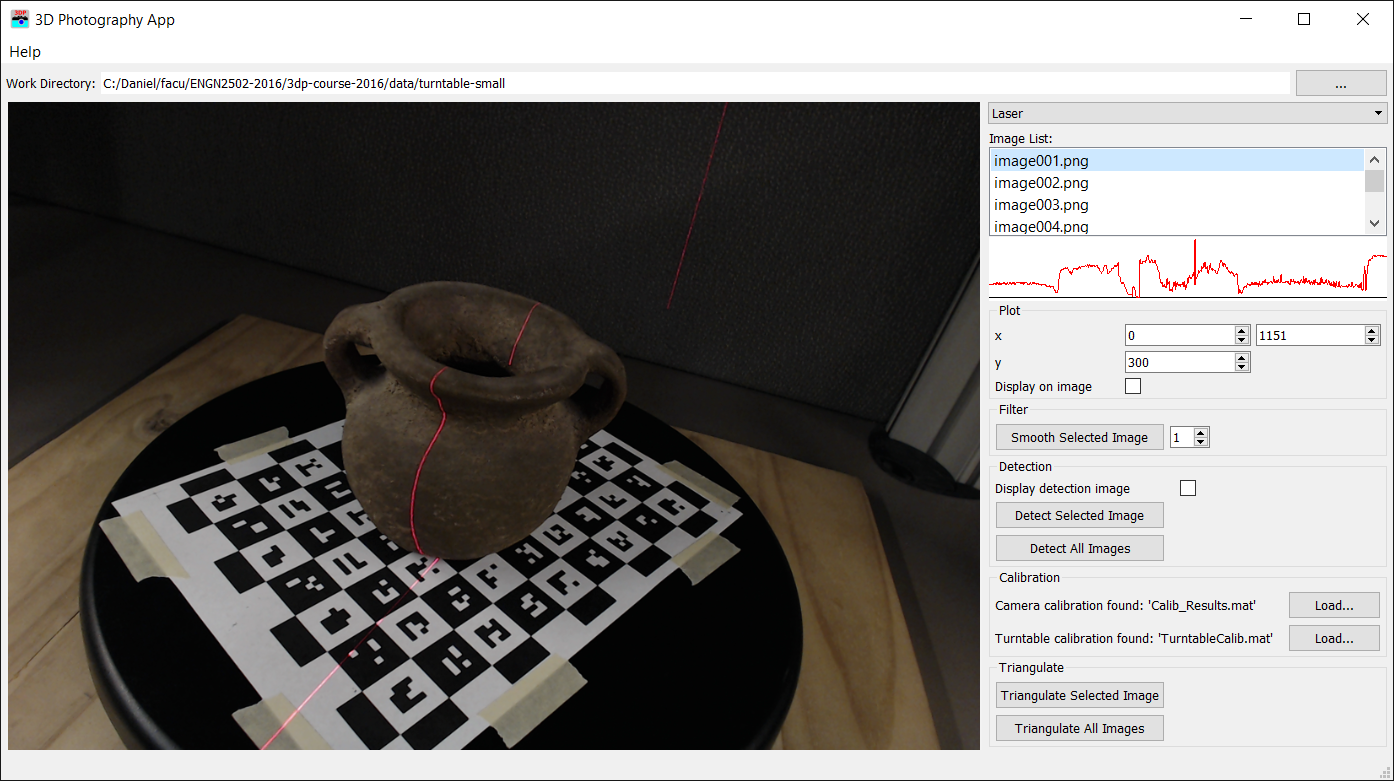
Figure 6: Laser Triangulation Panel
The triangulation function is called from the software by pressing the 'Triangulate Selected Image' or 'Triangulate All Images' buttons. When triangulation is completed a dialog will open to choose save a pointcloud.xyz file. This file is just a list of 3D points and can be visualized with a viewer such as Meshlab.
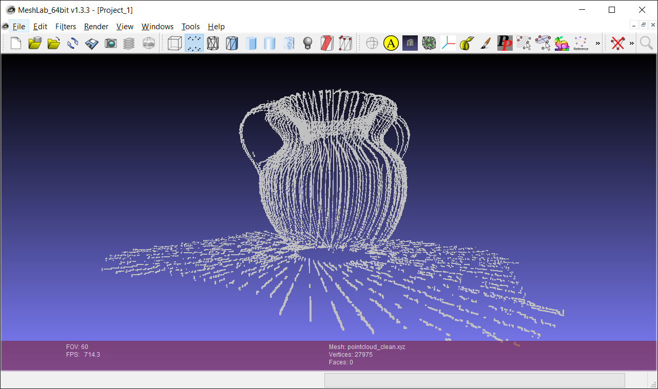
Figure 7: Pointcloud visualization in Meshlab
Submission Instructions
You must upload a Zip file of the complete application, including your implementation of the required functions, in canvas. If you need to communicate with the TA some implementation details, issues, exceptional results, extra work done, or anything else that you want to be considered while grading, do it so by writing a comment in the 'homework2.cpp' file, or add a document in the root folder of the software.
You must also include a folder called 'results' with the file 'pointcloud.xyz' resulting from triangulation of the turntable data. Do not forget to include also the files from your Camera calibration as detailed in 1.1, either in the same Zip file or as a separate one.
References
- G. Taubin and D. Moreno. Build Your Own Desktop 3D Scanner (Chap. 2 & 4). SIGGRAPH2014