
Assignment 3:
Turntable and Laser Plane Calibration
Instructor: Gabriel Taubin
Assignment developed by:
Daniel Moreno
and
Gabriel Taubin
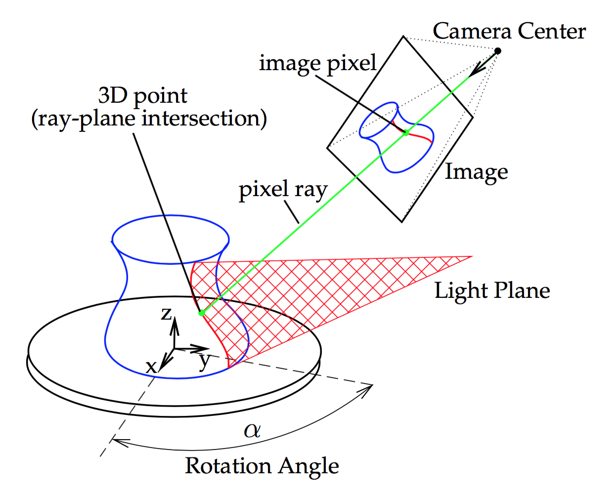
Figure 1: Laser Slit 3D Scanner setup.
Downloads
Download the new course software source files 3dp-course-2016-assignment3-1.0.zip . Remember to copy your homework1.hpp, homework1.cpp, homework2.hpp and homework2.cpp files into the src/homework directory. To perform the Turntable Calibration task download the following file CheckerboardCorners.mat or CheckerboardCorners.mat.zip and move into the directory where you saved the images used in assignment 2 data-turntable-small.zip . We will also need the calibration files for those images in the same directory turntable-small-calib.zip To perform the LaserPlane Calibration task download the following zip file containing the calibration images laser-plane.zip , download the following file Calib_Results.mat , or Calib_Results.mat.zip , and move into this new directory
Introduction
In a turntable-based 3D scanner, such as the one we are building, the world coordinate system is usually defined so that the origin is located at the intersection of the axis of rotation and the turntable plane, the z axis is aligned with the axis of rotation, the x and y axes span the turntable plane. In this assignment we will calibrate the turntable coordinate system by estimating the turntable plane and axis of rotation. We will also estimate the equation of the laser plane with respect to the camera coordinate system, which given the construction of our laser-based 3D scanner, does not change over time.
1 Turntable Calibration
A computer controlled turntable will provide us with the current rotation angle that corresponds to the stepper motor current rotation. Sometimes, as in the case of a manual turntable, that information is not available and the rotation must be computed from the current image. We will do so with the help of a CALTag checkerboard pasted flat on the turntable surface. The CALTag checkerboard assigns a unique code to each checkerboard cell which is used to identify the visible cells in an image even when a region of the checkerboard is occluded. We need this property because the target object sitting on top the turntable will occlude a large region of the CALTag. The corners of the visible checkerboard cells is a set of points rotating together with the turntable and will allow us to compute a rotation angle for each captured image.
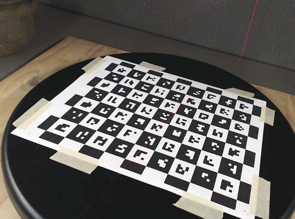
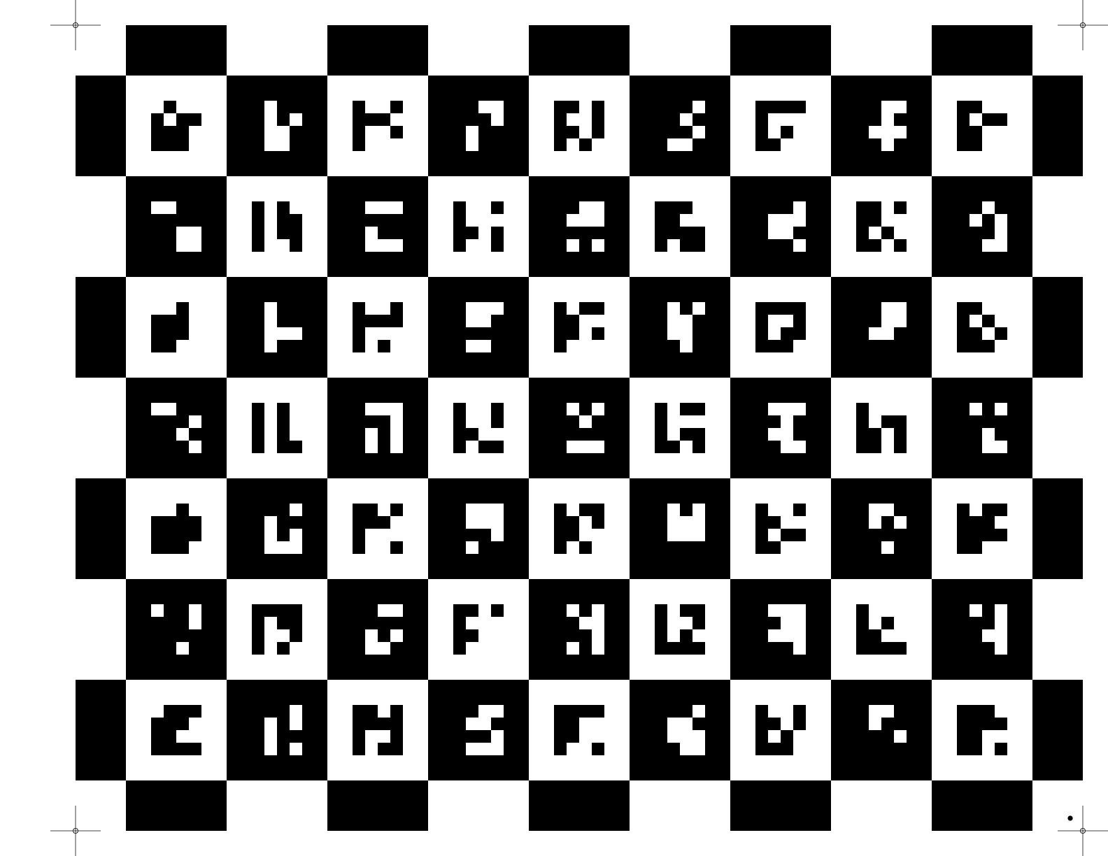
Figure 2: (Left) A CALTag checkerboard pasted on the turntable surface helps to recover the current rotation angle. (Right) Sample CALTag pattern.
At this point we assume the camera is calibrated and a set of images of the turntable at different rotations was captured. In addition, a set of 3D points on the turntable plane was identified in each image. Points coordinates are in reference to a known coordinate system chosen by the user. We will show how to find the unknown center of rotation and the rotation angle of the turntable for each image. In the current example, we align the coordinate system with the checkerboard and we identify the checkerboard and turntable planes with the plane $z=0$.
1.1 Camera Extrinsics
The first step is to find the pose of the camera for each image in reference to the known coordinate system. At this point we will compute a rotation matrix \(R\) and a translation vector \(T\) for each image independently of the others, such that if a point \(p\) in the reference system projects onto a pixel \(u\), they are related by the projection equation \(\lambda u = K (R p + T)\), where $$ R=\begin{bmatrix} r_{11}&r_{12}&r_{13}\\ r_{21}&r_{22}&r_{23}\\ r_{31}&r_{32}&r_{33} \end{bmatrix} \qquad T=\begin{bmatrix} T_x\\ T_y\\ T_z \end{bmatrix} $$
and \(u\), \(p\), and \(K\) are known. Point \(p = [p_x, p_y, 0]^T\) is on the checkerboard plane and \(u = [u_x, u_y, 1]^T\) is expressed in homogenous coordinates. We define the normalized pixel \(\tilde{u}=K^{-1}u\) and rewrite the projection equation as follows
$$ [0,0,0]^T = \tilde{u} \times (\lambda \tilde{u}) = \tilde{u} \times (R p + T) $$ $$ = \tilde{u} \times \begin{bmatrix} r_{11}p_x+r_{12}p_y+T_x\\ r_{21}p_x+r_{22}p_y+T_y\\ r_{31}p_x+r_{32}p_y+T_z \end{bmatrix} $$ $$ = \begin{bmatrix} \ \ \ \ -(r_{21}p_x+r_{22}p_y+T_y)&+&\tilde{u}_y(r_{31}p_x+r_{32}p_y+T_z)\\ \ \ \ \ \ \ \ (r_{11}p_x+r_{12}p_y+T_x)&-&\tilde{u}_x(r_{31}p_x+r_{32}p_y+T_z)\\ -\tilde{u}_y(r_{11}p_x+r_{12}p_y+T_x)&+&\tilde{u}_x(r_{21}p_x+r_{22}p_y+T_y) \end{bmatrix} $$Of these three equation only 2 are linearly independent, and it is easy to show that the first two eautions are always linearly independent. We select the first two equations and we group the unknowns in a vector \(X=[r_{11},r_{21},r_{31},r_{12},r_{22},r_{32},T_x,T_y,T_z]^T\), resulting in two equation for each point-pixel pair
$$ \begin{bmatrix} 0&-p_x&+\tilde{u}_y p_x & 0&-p_y&+\tilde{u}_y p_y & 0&-1&+\tilde{u}_y\\ p_x& 0&-\tilde{u}_x p_x &p_y& 0&-\tilde{u}_x p_y & 1& 0&-\tilde{u}_x \end{bmatrix} X = \begin{bmatrix}0\\0\end{bmatrix}. $$Until now we have considered a single point \(p\), but in general, we will have a set of points \(\{\,p_1,\ldots p_N\}\) for each image, with corresponding normalized pixels \(\{\tilde{u}_1,\ldots,\tilde{u}_N\}\). In this assignment we assume that the points have already been detected, and their cooresponding pixel coordinates have been measured, but in general determining which points are visible in each image, and measuring their pixel coordinates constitutes an additional step. Note that the number \(N\) of visible points changes from image to image. We use all the points from all the images to build a single system of homogeneous linear equations \(AX=0\) where \(A \in \mathbb{R}^{2n\times 9}\) contains 2 rows as in the previous equation for each point \(p_i\) stacked together, and we solve
$$ \hat{X} = arg\min_X ||AX||,\ \ \ \text{s.t.} \ \ ||X|| = 1 $$We constrain the norm of X in order to get a non-trivial solution. Vector \(X\) has 8 degrees of freedom, thus, matrix \(A\) must be rank 8 so that a unique solution exists. Therefore, we need at least 4 non-collinear points in order to get a meaningful result. After solving for \(\hat{X}\) we need to rebuild \(R\) as a rotation matrix.
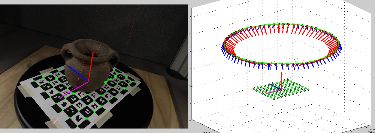
$$ \hat{r_1} = [r_{11},r_{21},r_{31}]^T, \ \hat{r_2} = [r_{21},r_{22},r_{23}]^T, \ \hat{T} = [T_x,T_y,T_z]^T, s = \frac{2}{||\hat{r_1}||+||\hat{r_2}||} $$ $$ r_1 = s\,\hat{r_1}, \ r_3 = r_1\times s\,\hat{r_2}, \ r_2 = r_3 \times r_1 $$ $$ R = \begin{bmatrix}r_1&r_2&r_3\end{bmatrix}, \ T = s\,\hat{T} $$Figure 3 shows our software running the camera extrinsics computation as described here.
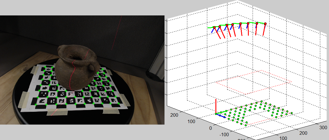
Figure 3: Screenshot of the supplied software running camera extrinsics computation. (Left) Image being processed: identified CALTag corners displayed in green. (Right) 3D view: CALTag corners shown in green below, cameras displayed above with their $z$-axis on red, the reference coordinate system was set at the origin of the checkerboard.
1.2 Center of Rotation and Rotation Angle
In the previous section we showed how to estimate \(R_k\) and \(T_k\) for each of the \(N\) cameras independently. Now, we will use the fact that the turntable rotates in a plane and has a single degree of freedom to improve the computed camera poses. We begin finding the center of rotation \(q=[q_x,q_y,0]^T\) in the turntable plane which must satisfy the projection equations as any other point
$$ \lambda_k \tilde{u}_k = R_k q + T_k $$By definition of rotation center its position remains unchanged before and after the rotation, this observation allow us to define \(Q\equiv\lambda_k \tilde{u}_k,\ \forall k\), and write
$$ R_k q + T_k = Q $$ $$ \begin{bmatrix}R_1&-I\\R_2&-I\\\vdots&\vdots\\R_N&-I\end{bmatrix} \begin{bmatrix}q\\Q\end{bmatrix} = \begin{bmatrix}-T_1\\-T_2\\\vdots\\-T_N\end{bmatrix} \ \Rightarrow\ AX=b $$ $$ \hat{X} = arg\min_X ||AX-b|| $$In order to fix \(q_z=0\), we skip the third column in the rotation matrices reducing \(A\) to 5 columns and changing \(X = [q_x,q_y,Q_x,Q_y,Q_z]^T\).
Let be \(\alpha_i\) be the rotation angle of the turntable in the \(i\)-th image,
then for every \(1,\leq k
The turntable position in the first image is designated as the origin:
\(\alpha_1=0\). We get an approximate value for each other \(\alpha_k\)
by reading the values \(\cos\alpha_k\) and \(\sin\alpha_k\) from \(R_1^T
R_k\) and setting
Figure 4 shows the center of rotation
obtained with this method drawn on top of an input image and its
corresponding 3D view.
Figure 4: Center of rotation. (Left) Camera image: center of rotation
drawn on top. (Right) 3D view: world coordinate system at the center
of the rotation.
The final step in turntable calibration is to refine the values of all
the parameters using a global optimization. The goal is to minimize
the reprojection error of the detected points in the images
where and
\(J_k\) is the subset of checkerboard corners visible in image \(k\),
\(\alpha_1 = 0\), and \(u_k^i\) is the pixel location corresponding to
\(p_i\) in image \(k\). We begin the optimization with the values \(q\),
\(R_1\), \(o_1=-R_1^T T_1\), and \(\alpha_k\) found in the previous sections
which are close to the optimal solution.
The new file CheckerboardCorners.mat contains the 2D coordinates of
the visible checkerboard corners is the local coordinate system of the
checkerboard, as well as pixel coordinates of the corresponding image
points. The intrinsic calibration is read from the file
Calib_Results.mat that you used in the previous assignments. We also
need the TurntableCalib.mat in the same directory. In this assignment
you will override some of the precomputed values in these files. A
new group was added to the Laser panel, in the course software, to use
the methods that you will implement in this assignment.
You need to implement the following method to estimate the camera
extrinsic parameters for each image, using the method described in
section 1.1. The method is called by when the "Calibrate Selected" or
"Calibrate All" pushbuttons are pressed. The resulting translation and
rotation is saved in the data structure containg the data read from
the CheckerboardCorners.mat file
Once all the rotations and translations are computed by running the
previous method on all the input images, the "Estimate Center" button
is enabled. You have to implement the following method to estimate the
center of rotation of the turntable. The center of rotation is
represented by its two coordinates with respect one of the
checkeboards. Note that the checkerboard coordinates of the center
should be the same for all the images. In this method you should also
compute the world coordinates rotation and translation. Remember that
the world rotation is the rotation corresponding to the first image,
and the worl translation is the loaction of the turntable center in 3D
with respect to the camera coordinate system.
You also have to implement the following method to verify that your
computations are correct. This is a modified version of the method
with the same name that you implemente in homework 2. One difference
is that the world points are not three dimensional, but two
dimensional here, since all the checkerboard points have the third
coordinate equal to zero. You also have to add the conversion of those
points to world coordinates, and save the results in the provided
worldPonts array. This method is called when the "Save Turntable
Points" pushbutton is pressed, which is enabled after the center of
rotation has been computed.
Finally, we need to calibrate the location of the plane of light
generated by the laser. The calibration consists in identifying some
points we know belong to the plane and finding the best plane, in the
least squares sense, that matches them. The projection of the laser
line onto the turntable provides us with a set of such points,
however, they are all in a straight line and define a pencil of planes
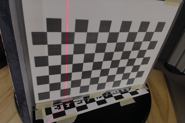
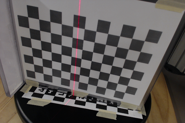
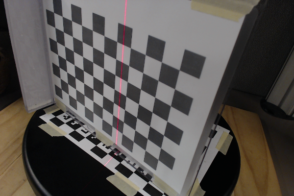
rather a single plane. An easy way to find additional points is to place
a checkerboard plane onto the turntable and capture images at several
rotation angless, as shown in Figure 5.
Figure 5: Light plane calibration: an extra plane is placed onto the
turntable and is rotated to provide a set of non-collinear points.
The orientation of the camera with respect to the checkerboard plane
is calculated with the method from Section 1.1. The laser pixels are
identified with the detection algorithm and they are triangulated
using ray-plane intersection providing a set of 3D points on the
checkerboard plane. We can choose to triangulate the laser points on
the turntable plane too, which makes possible to calibrate with a
single image. It is recommendable to capture additional images to have
more samples of the light plane for a better calibration. In particular,
we would like samples at different depths in the scanning
volume. Checkerboard images captured for the camera intrinsic
calibration can also be reused to calibrate the plane of light, this way no
extra images are required. This idea is illustrated in Figure 6.
Figure 6: Light plane calibration result. A checkerdboard plane was
placed on the turntable and images at several rotations were
captured. Images are used first for camera calibration, and later for
calibration of the light plane (shown in orange).
The Laser panel also has a new "Laser Plane Calibration" group. The
software reads the checkerboard corner coordinates and corresponding
pixel coordinates from the "Results_Calib.mat" file and provides them
to you. When you press the "Reconstruct Selected" or the "Reconstruct
All" pushbuttons, the "estimateExtrinsics()" method is first called to
estimate the rotation and translation for that particular
checkerboard.
Based on what you did in homework 1, you should implement the
following method to detect the points illuminated by the laser. Rather
than an image showing the detected pixels, the here result should be a
vector of 2D pixel coordinates.
Since we also need the equation of the checkerboard plane, you should
implement the following method to estimate the implicit equation of
the checkerboard plane in the camera coordinate system. The method
takes as input the rotation and translation returned by the
"estimateExtrinsics()" method.
Now we can triangulate the pixels returned by the new "detectLaser()"
method. You should implement the following method to do so. Keep in
mind that lens distortion has not been removed from the pixel
coordinates yet. The method should return a vector of 3D points in
camera coordinates, which should be on the checkerboard plane.
Finally, you need to fit a plane to the collected points using the
eigenvector method discussed in class, and return the coefficients of
the implicit equation as a four dimensional vector. The "laserPoints"
point cloud will be saved as a file named "laserpoints.xyz" which you
will have to submit along with your code.
1.3 Global Optimization
1.3 Turntable Calibration Tasks
void hw3::estimateExtrinsics(Matrix3d const& K, /* intrinsic */
Vector5d const& kc, /* intrinsic */
QVector
void hw3::estimateTurntableCenter(QVector
double hw3::reprojectPoints(Matrix3d const& K, /* input */
Vector5d const& kc, /* input */
Matrix3d const& R, /* input */
Vector3d const& T, /* input */
QVector 2 Laser Plane Calibration

2.1 Laser Plane Calibration Tasks
void hw3::detectLaser(QImage const& inputImage,
QVector
  void hw3::checkerboardPlane(Matrix3d& R, /* input */
                              Vector3d& T, /* input */
                              Vector4d const& checkerboardPlane /* output */);
void hw3::triangulate(Matrix3d const& K, /* input */
Vector5d const& kc, /* input */
Vector4d& planeCoefficients, /* input */
QVector
void hw3::estimatePlane(QVector
3 Submission Instructions
You must upload a Zip file of the complete application, including your implementation of the required functions, in canvas. If you need to communicate with the TA some implementation details, issues, exceptional results, extra work done, or anything else that you want to be considered while grading, do it so by writing a comment in the 'homework2.cpp' file, or add a document in the root folder of the software.
You must also include a folder called 'results' with the file 'turntablepoints.xyz' resulting from pressing the "Save Turntable Points" pushbutton, and the 'laserpoints.xyz' resulting from pressing the "" pushbutton.
References
- G. Taubin and D. Moreno. Build Your Own Desktop 3D Scanner (Chap. 4). SIGGRAPH2014