Assignment 5:
Automated Image-Stitching
The goal of this assignment is to implement several software components that allows to automatically align and stitch two images with overlapping field of view to produce a single image.
DATES
The assignment is out on Friday, November 16, 2012, and it is due on Friday, November 30, 2012.
ASSIGNMENT FILES
Download the zip file ENGN1610-2012-A5.zip containing all the Assignment 3 files. Unzip it to a location of your choice. You should have now a directory named assignment5 containing a number of files, including all the files which you modified in previous assignments, as well as
- Makeflie
- JImgShopA5.zip
- JImgShopA5.lnk
- JImgPanelPanoramas.java
- ImgPanoramas.java
OVERVIEW
In this assignment you will be implementing a very simplified version of the automated image stitching software described in "Multi-Image Matching using Multi-Scale Oriented Patches". The input of our software is a pair a images with some overlap and the output is one (larger) image made by aligning and blending the input images together. We will split the process in the following steps:
- Feature detection
- Feature matching
- Computing the matching transformation
- Image stitching
FEATURE DETECTION
In
this step you will be implementing the Harris corner detector. Given
the auto-correlation matrix \(A\)
of the image
\[
A=G*\left[\matrix{I_x^2 & I_xI_y\cr I_xI_y &
I_y^2}\right]
\]
where \(I_x\) and \(I_y\) are the image intensity derivatives, and
\(G\) is a Gaussian kernel, the Harris-Stephens corner score \(R\) is
defined as
\[ R=Det(A)-\alpha\, Trace(A)^2 \]
A point \( (x,y) \) in the image is a corner if
\(R(x,y)>threshold\), the constant \(\alpha\) is a sensitivity
parameter (e.g. \(0.04\)).
public void detectKeypoints(Img srcImg, int imgId, float threshold)
Complete the function detectKeypoints() to compute the Harris score \(R\) for each pixel and if \(R>threshold\) add an element to the keypoint list _keyPts[imgId]. The parameter imgId maybe be 0 or 1 meaning the left or right image. You can approximate \(I_x\) and \(I_y\) by convolving the image with the Sobel operator or directly by \[I_x(x,y)=\frac{I(x+1,y)-I(x-1,y)}{2}, \ \ \ I_y(x,y)=\frac{I(x,y+1)-I(x,y-1)}{2} \]
A simple way of computing the Harris score for each pixel is to build a temporary image with \(I_x^2\),\(I_y^2\), and \(I_xI_y\) (e.g. store \(I_x^2\) in the red channel, \(I_y^2\) in the channel, and \(I_xI_y\) in the blue channel) and convolve this image with a Gaussian. Then recover the values from the convolved image and compute \(R\) using the formula above. Finally, compare the score with the provided threshold value to decide if there is a corner at that location or not. You may call the provided function blurImage() to convolve an image with a Gaussian.
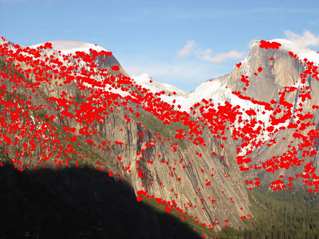
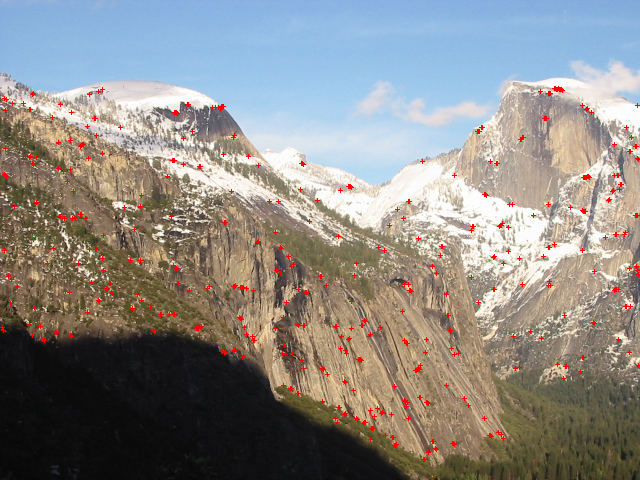
If you do this correctly, you may get thousands of corners for each image. In order to reduce the number of corners to process and to distribute them evenly in the image, the list of keypoints will be filtered using Adaptive Non-maximal Suppression (ANMS). ANMS is already implemented in the starting code. You can set the maximum number of keypoints you want to keep in the GUI and the algorithm will automatically select them in an optimal way.
| All corners | Corners after ANMS (N=500) |
 |
 |
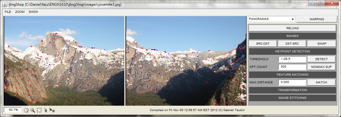
FEATURE MATCHING
Now that we have detected the keypoints, we want to determine their correspondences between images. You can be creative here but for our simplified scheme just comparing all keypoints from one image to the keypoints of the other by brute-force will work fine.
The comparison can be made by taking a patch (e.g. \(5\times5\)) around each of the keypoint locations and comparing their pixels with some distance function. If the distance is smaller than some value, the keypoints are set as a match. Again, in our simplified setup, we do not expect large variations in scale, rotation, or intensity between images, and a simple distance as the Sum of Squares Differences will give good results in general. You can choose to implement SSD or some other distance function.
Independently of the distance function used, we expect to be many wrong matches. One way to reduce the number of wrong matches is to search the first and second matching keypoints (the one with the minimum distance and the one with the second minimum distance) and to set them as a match if and only if the distance between them is large. For example, let \(kpt1\) be a keypoint in image 1 and \(kpt2\) and \(kpt3\) its first and second matches in image 2, we say that \((kpt1,kpt2)\) are a match if \[dist(kpt1,kpt2)<0.7*dist(kpt1,kpt3)\]
public void matchKeypoints(float minDist)
Complete the function matchKeypoints(). Keypoints in both images will be already extracted and stored in the member variable _keyPts[imgId] (imgId is 0 or 1) and your task is to compare them using some distance measure and save the matches in _matches member variable. You should add two numbers to _matches for each match: the first number is the Id of the keypoint in the first image and the second the Id of the second keypoint.
REMOVING OUTLIERS AND COMPUTING THE MATCHING TRANSFORMATION
The matches found in the previous step are our correspondences between image locations. The next step is to use these correspondences to compute a transformation between images. Here you will be computing a homography \(H\) such that \[X_1=H\,X_2\ , \ \ \ \left[\matrix{x_1 \cr y_1 \cr w_1}\right] = \left[\matrix{h_0 & h_1 & h_2 \cr h_3 & h_4 & h_5 \cr h_6 & h_7 & 1}\right]\,\left[\matrix{x_2 \cr y_2 \cr 1}\right] \]
\(H\) has 8 dof and it is defined up-to-scale. Given 4 points correspondences there is an exact solution (if there no 3 colinear points among them).
We have our point correspondences from the previous step (usually many more than 4!), but many of them might not be correct. You will have to solve for the homography that agree with most of the matches using RanSaC (Random Sample Consensus). The pseudocode for RanSaC is the following:
\(N\) = number of iterations
\(outliers = 0\)
\(H, minOutliers\)
Repeat \(N\) times
- Select \(4\) matches randomly
- Compute a homography \(\bar{H}\) using the keypoint locations from the matches
- For each match
\(err = \|X_1 - \bar{H}\,X_2\|^2\)
If \(err>1\) then: \(outliers = outliers + 1\)
- If \(outliers < minOutliers\) then: \(H=\bar{H}, minOutliers = outliers\)
Return \(H\)
The output of the algorithm is the homography \(H\) with a small number of outliers between all the matches found. To learn how to compute \(H\) (and its inverse) directly from the point correspondences you may read "Projective Mappings for Image Warpings".
public void computeTransformation()
Write your implementation of RanSaC in computeTransformation(). Store the final homography in the member variable _transform.
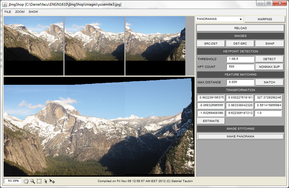
IMAGE STITCHING
The last step is just creating a new image with both images aligned. If you did correctly the previous assignments this part should be really easy.
public Img makePanorama()
Complete makePanorama() to create a new images blending the pixels from both images accordingly to the found homography.