
Assignment 1: 3D Photography with Planar Shadows
Instructor: Gabriel Taubin
Assignment developed by: Douglas Lanman
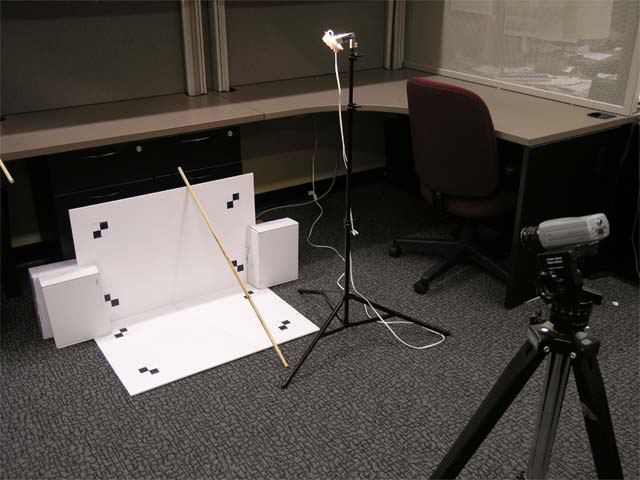
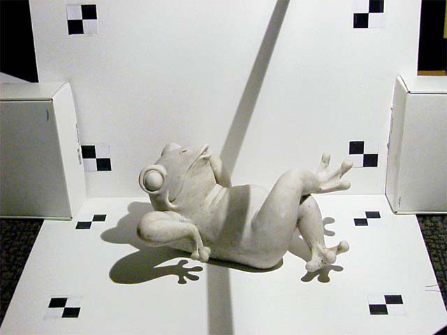
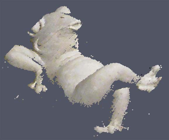
Figure 1: 3D Photography using Planar Shadows. From left to right: the capture setup, an image from the scanning sequence, and a reconstruction (rendered as a colored point cloud).
Downloads: handout, support code
Sequences: calibration, chiquita, frog, man, schooner, urn, yong
Introduction
The goal of this assignment is to build an inexpensive, yet accurate, 3D scanner using household items and a camera. Specifically, we'll implement the "desktop scanner" originally proposed by Jean-Yves Bouguet and Pietro Perona [3]. As shown in Figure 1, our instantiation of this system is composed of five primary items: a camera, a point-like light source, a stick, two planar surfaces, and a calibration checkerboard. By waving the stick in front of the light source, the user can cast planar shadows into the scene. As we'll demonstrate in this handout, the depth at each pixel can then be recovered using simple geometric reasoning.
In the course of completing this homework, you will need to develop a good understanding of camera calibration, Euclidean coordinate transformations, manipulation of implicit and parametric parameterizations of lines and planes, and efficient numerical methods for solving least-squares problems. Before you begin this assignment, you should first browse the original project website [3] and obtain a copy of the IJCV publication [4] – which we'll reference several times in this document.
1 Data Capture
This assignment does not require you to construct the actual scanning apparatus. Instead, we have provided you with nine test sequences collected using our setup. As shown in Figures 3-10, there are a variety of objects available – ranging from those with smooth surfaces to those with multiple self-occlusions. As we'll describe in the following sections, reconstruction requires accurate estimates of the of shadow boundaries. As a result, you will find that light-colored objects (e.g., the chiquita, frog, and man sequences) will be easiest to reconstruct. Since you'll need to estimate the intrinsic and extrinsic calibration of the camera, we've also provided the calib sequence composed of ten images of a checkerboard at various poses. All of these sequences can be obtained on the course website. Note that the frog and calib sequences are included in the /data directory of the support code package. For each sequence we have provided both a high-resolution 1024x768 sequence, as well as a low-resolution 512x384 sequence for development.
Before you proceed, briefly note some practical issues associated with this approach. First, it is important that every pixel be shadowed at some point in the sequence. As a result, you must wave the stick slow enough to ensure that this condition holds. In addition, the reconstruction method requires reliable estimates of the plane defined by the light source and the edge of the stick. Ambient illumination must be reduced so that a single planar shadow is cast by each edge of the stick. In addition, the light source must be sufficiently bright to allow the camera to operate with minimal gain – otherwise sensor noise will corrupt the final reconstruction. Finally, we note that these systems typically use a single halogen desk lamp with the reflector removed. This ensures that the light source is sufficiently point-like to produce abrupt shadow boundaries. Otherwise, the estimate of the shadow plane will not be reliable. Once you complete this assignment you may be inspired to build your own apparatus – keep these observations in mind.
2 Video Processing
If you've had a chance to review the IJCV publication [4], then you'll realize that we must begin by estimating two fundamental quantities from an input video sequence: (1) the time that a shadow enters a pixel and (2) the position of the shadow edge as a function of time. The following sections outline the basic procedures for performing these tasks. Please consult Section 2.4 in [4] or Section 6.2.4 in [2] for additional information.
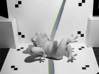
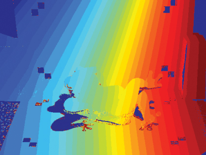
Figure 2: Spatial and temporal shadow edge localization. (a) The shadow edges are determined by fitting a line to the set of zero crossings, along each row in the planar regions, of the difference image ΔI(x,y,t). (b) The shadow times are determined by finding the zero-crossings of the difference image ΔI(x,y,t) for each pixel (x,y) as a function of time t.
2.1 Spatial Shadow Edge Localization
In terms of Figure 2 in [4], we need to estimate the shadow lines λh(t) and λv(t) projected on the horizontal and vertical planar regions, respectively. In order to perform this and subsequent processing, we utilize a spatio-temporal approach. As described in the references, this approach tends to produce better reconstruction results than traditional edge detection schemes (e.g., the Canny edge detector [5]), since it is capable of preserving sharp surface discontinuities.
We begin by defining the maximum and minimum brightness observed in each pixel (x,y), given by Imax(x,y) and Imin(x,y). In order to detect the shadow boundaries, we choose a per-pixel detection threshold which is the midpoint of the dynamic range observed in each pixel. As a result, the shadow edge can be localized by the zero crossings of the difference image ΔI(x,y,t) = I(x,y,t) - Ishadow(x,y), where the shadow threshold image is defined to be Ishadow(x,y) = (Imax(x,y) + Imin(x,y))/2.
In practice, you'll need to select an occlusion-free image patch for each planar region. Afterwards, you can obtain a set of sub-pixel shadow edge samples (for each row of the patch) by interpolating the position of the zero-crossings of ΔI(x,y,t). To produce a final estimate of the shadow edges λh(t) and λv(t), you should find the best-fit line (in the least-squares sense) to the set of shadow edge samples. The desired output of this step is illustrated in Figure 2(a), where the best-fit lines are overlaid on the original image. Keep in mind that you should convert the provided color images to grayscale; if you're using Matlab, the function rgb2gray can be used for this task.
2.2 Temporal Shadow Edge Localization
After calibrating the camera, the previous step will provide all the information necessary to recover the position and orientation of each shadow plane as a function of time. As we'll describe in Section 4, in order to reconstruct the object we also need to know when each pixel entered the shadowed region. This task can be accomplished in a similar manner as spatial localization. Instead of estimating zero-crossing along each row for a fixed frame, we'll assign the per-pixel shadow time using the zero crossings of the difference image ΔI(x,y,t) for each pixel (x,y) as a function of time t. The desired output of this step is illustrated in Figure 2(b), where the shadow crossing times are quantized to 32 values (with blue indicating earlier times and red indicated later ones). Note that you may want to include some additional heuristics to reduce false detections. For instance, dark regions cannot be reliably assigned a shadow time. As a result, you can eliminate pixels with insufficient contrast.
3 Calibration
As discussed in class, you will require the intrinsic and extrinsic calibration of the camera in order to transfer image measurements into the world coordinate system. For this assignment we will be using the Camera Calibration Toolbox for Matlab, also created by Jean-Yves Bouguet. This toolbox is widely used within the computer vision community and, at its core, implements a similar method as proposed by Zhengyou Zhang [6]. That is, the intrinsic and extrinsic parameters are estimated by viewing several images of a checkerboard at various poses. Before continuing, you should briefly review the documentation on the toolbox website [1]. In particular, review the first calibration example and the description of calibration parameters.
3.1 Intrinsic Calibration
The intrinsic parameters of the camera can be obtained using the calib sequence. Begin by adding the toolbox, located in /TOOLBOX_calib, to your Matlab path by selecting "File, Set Path...". Next, change the current working directory to one of the calibration sequences (e.g., /data/calib or /data/calib-lr). Type calib at the Matlab prompt to start. Since we're only using a few images, select "Standard (all the images are stored in memory)" when prompted. To load the images, select "Image names" and press return, then "j". Now select "Extract grid corners", pass through the prompts without entering any options, and then follow the on-screen directions. (Note that we used a calibration target with the default 30mm x 30mm squares. Also, always skip any prompts that appear.) Once you've finished selecting corners, choose "Calibration" – which will run one pass though the calibration algorithm we discussed in class. Next, choose "Analyze error". Left-click on any outliers you observe, then right-click to continue. Repeat the corner selection and calibration steps for any outliers (this is a manually-assisted form of bundle adjustment). Once you have an evenly-distributed set of reprojection errors, select "Recomp. corners" and finally "Calibration". To save your intrinsic calibration, select "Save".
3.2 Extrinsic Calibration
From the previous step you now have an estimate of how pixels can be converted into normalized coordinates (and subsequently rays in world coordinates, originating at the camera center). In order to assist you with your implementation, we have provided a Matlab script called extrinsicDemo. As long as the calibration results have been saved in /data/calib and /data/calib-lr, this demo will allow you to select four corners on the "horizontal" plane to determine the Euclidean transformation from this ground plane to the camera reference frame. (Always start by selecting the corner in the bottom-left and proceed in a counter-clockwise order. For your reference, the corners define a 558.8mm x 303.2125mm rectangle.) In addition, observe that the final section of extrinsicDemo uses the included function pixel2ray to determine the optical rays (in camera coordinates), given a set of user-selected pixels. While we've provided this demonstration, please describe in your documentation how you can convert from pixel coordinates to a ray in world coordinates.
4 Reconstruction
At this point you have estimated all the parameters required to recover the depth of each pixel in the image (or at least those where the shadow could be observed). In terms of Figure 2 in [4], you can use the camera calibration to obtain a parametrization of the ray defined by a true object point P and the camera center O. Given the shadow time for the associated pixel x, you can lookup (and potentially interpolate) the position of the shadow plane at this time. The resulting ray-plane intersection will provide an estimate of the 3D position of the surface point. Repeating this procedure for every pixel will produce a 3D reconstruction. For more details on the reconstruction process, please consult Sections 2.5 and 2.6 in [4] and Sections 6.2.5 and 6.2.6 in [2].
5 Post-processing and Visualization
Now that you've recovered a 3D point cloud, you will need to visualize the result. Regardless of the environment you used to develop your solution, you should write a function to export the recovered points as a VRML file containing a single indexed face set with an empty coordIndex array. Since we are not requiring you to create a polygonal mesh representation, you should assign per-vertex colors to "texture" the point cloud.
To give you some expectation of reconstruction quality, Figures 3-10 show the results obtained with our reference implementation. Note that there are several choices you can make in your implementation; some of these may allow you to obtain additional points on the surface or increase the reconstruction accuracy. Please document the methods you used to optimize your reconstruction.
Submission Instructions
You should submit clear evidence that you have successfully implemented the "desktop scanner". In particular, you should submit: (1) an archive named 3DPGP-HW1-Lastname.zip containing your source code without the /data directory, (2) a typeset document explaining your implementation, and (3) a set of reconstructed point clouds as VRML files. Final solutions should be emailed to the Instructor at taubin@brown.edu. (Please note that we reserve the right to request a 15 minute demonstration if the submitted documentation is insufficient to compile and run your solution.)
At a minimum, the included documentation should contain some images similar to Figure 2 – demonstrating that you were able to reliably estimate the spatial and temporal shadow edges (for a sequence besides frog-v1). To demonstrate that you were able to calibrate the camera, include your estimates (and short descriptions) of the intrinsic parameters: fc, cc, alpha_c, kc. Please provide a description of your specific reconstruction approach (e.g., how you parameterized various quantities and recovered the per-pixel depth). You should include at least one figure showing a reconstruction, and at least three different reconstructions as VRML files. If you didn't use Matlab, please provide brief instructions on compiling your solution. In any case, include a README file with a short description of every file (except those we provided) in 3DPGP-HW1-Lastname.zip.
References
- Jean-Yves Bouguet. Camera calibration toolbox for matlab. http://www.vision.caltech.edu/bouguetj/calib doc/.
- Jean-Yves Bouguet. Visual methods for three-dimensional modeling. PhD thesis, California Institute of Technology, 1999.
- Jean-Yves Bouguet and Pietro Perona. 3d photography on your desk. http://www.vision.caltech.edu/bouguetj/ICCV98/.
- Jean-Yves Bouguet and Pietro Perona. 3d photography using shadows in dual-space geometry. Int. J. Comput. Vision, 35(2):129{149, 1999.
- Yi Ma, Stefano Soatto, Jana Kosecka, and S. Shankar Sastry. An Invitation to 3-D Vision. Springer, 2005.
- Zhengyou Zhang. Flexible camera calibration by viewing a plane from unknown orientations. In International Conference on Computer Vision (ICCV), 1999.
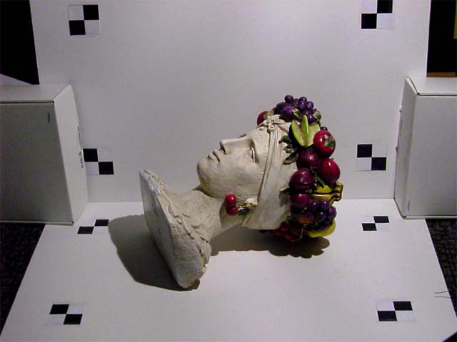
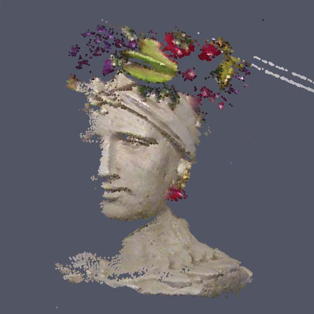
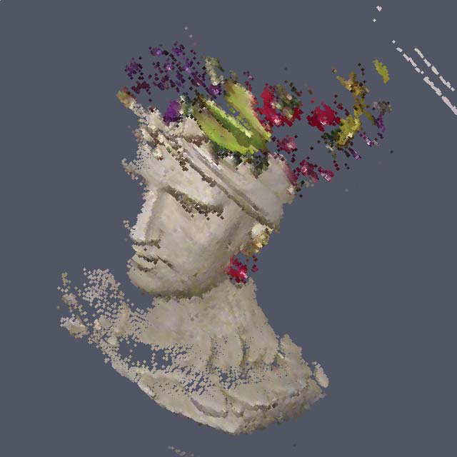
Figure 3: Reconstruction results for chiquita-v1 sequence.
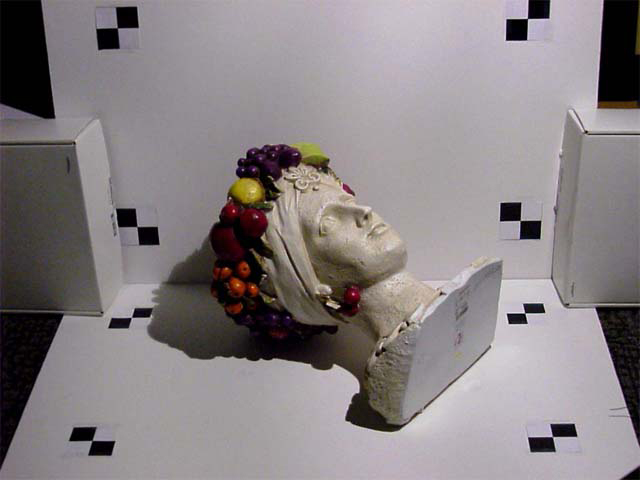
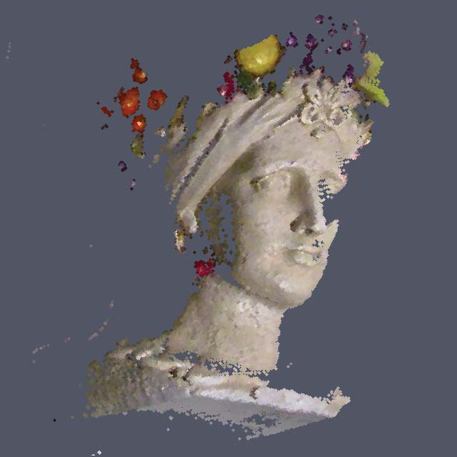
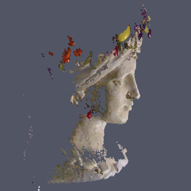
Figure 4: Reconstruction results for chiquita-v2 sequence.
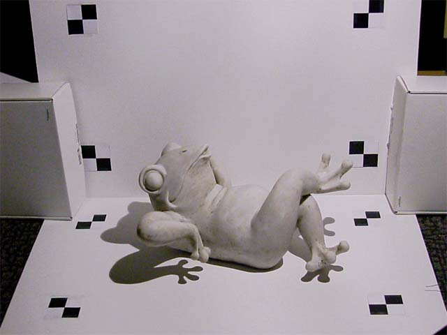
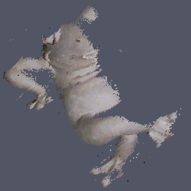
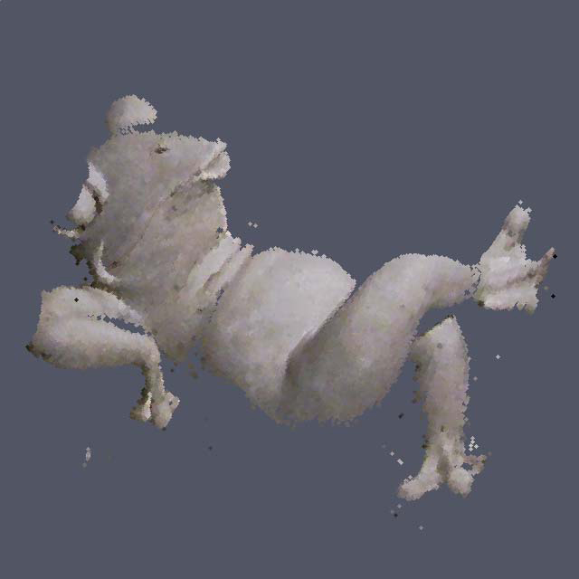
Figure 5: Reconstruction results for frog-v1 sequence.
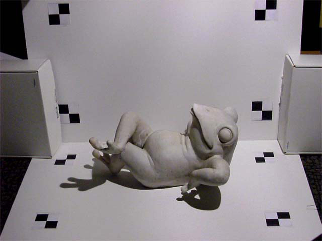
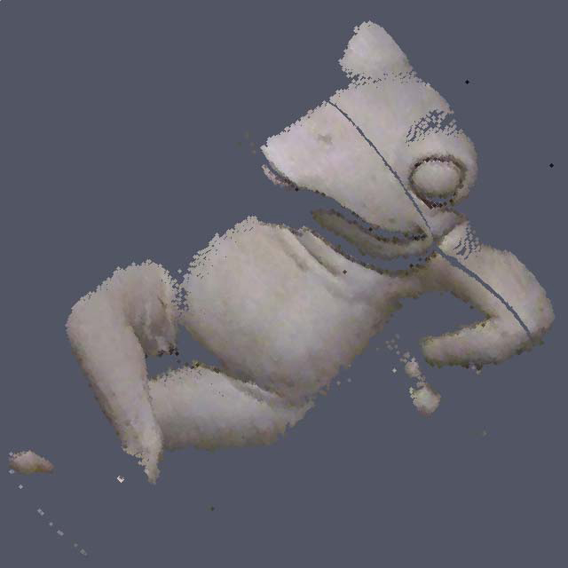
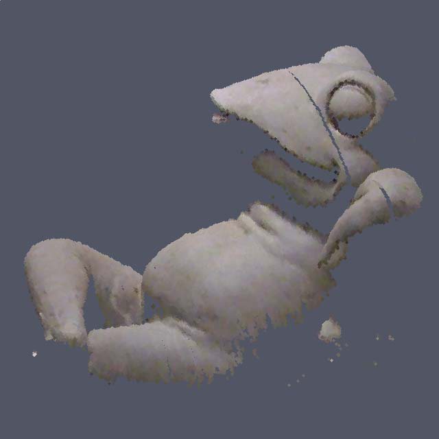
Figure 6: Reconstruction results for frog-v2 sequence.
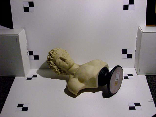
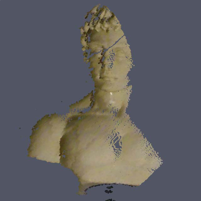
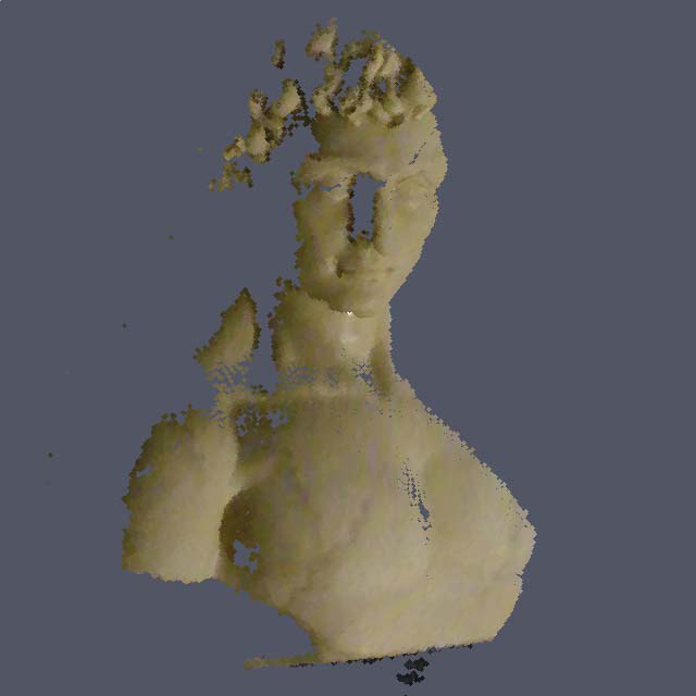
Figure 7: Reconstruction results for man-v1 sequence.
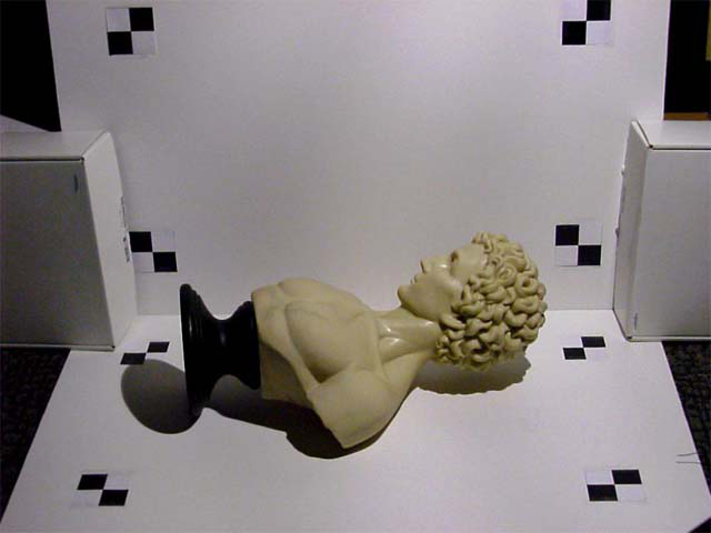
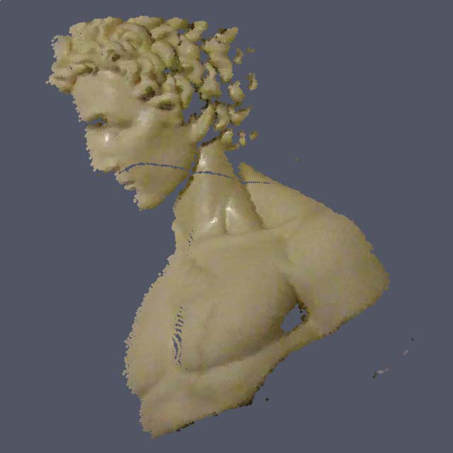
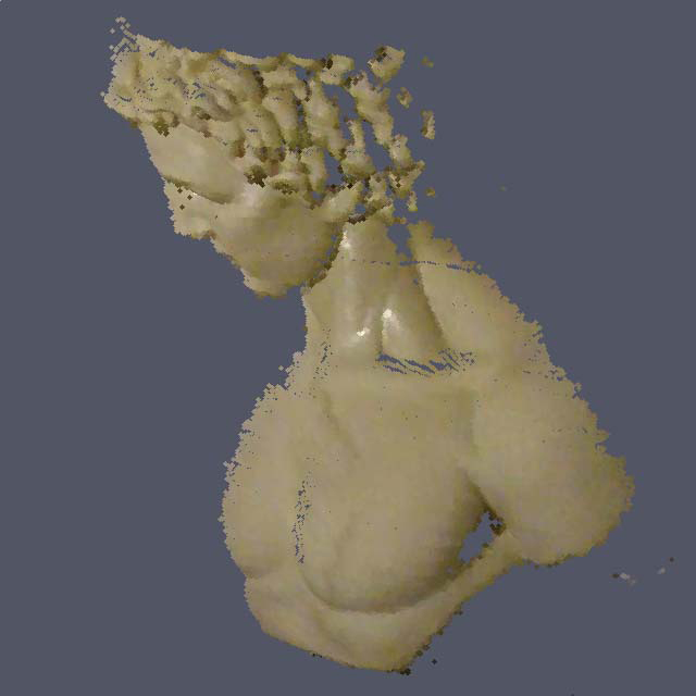
Figure 8: Reconstruction results for man-v2 sequence.
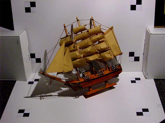
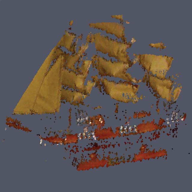
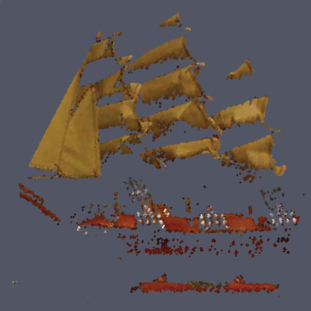
Figure 9: Reconstruction results for schooner sequence.
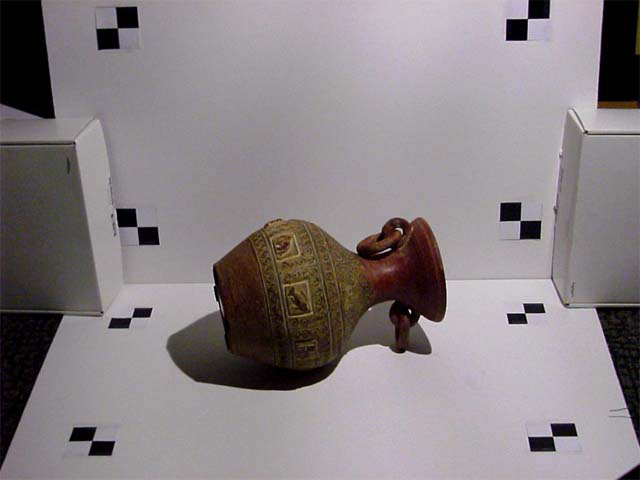
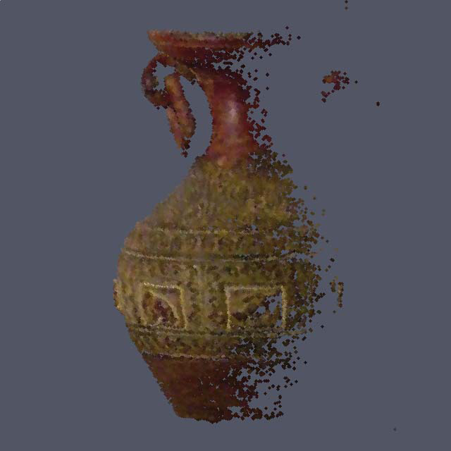
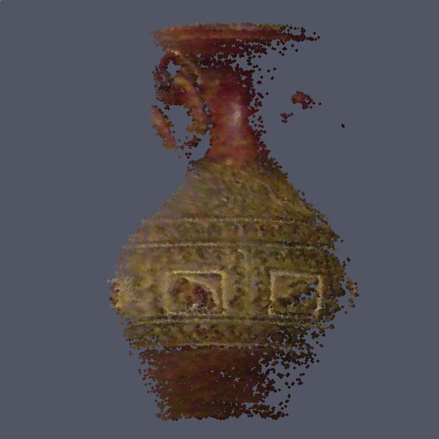
Figure 10: Reconstruction results for urn sequence.