
US Patent No. US10417822B2
Non-Convex Hull Surfaces
by Gabriel TaubinGranted on 09/17/2019
Download: US10417822B2.pdf
US Patent No. US10445400B2
Non-Convex Hull Surfaces
by Gabriel TaubinGranted on 09/15/2019
Download: US10445400B2.pdf
Fast Non-Convex Hull Computation
by Julián Bayardo Spadafora, Francisco Gómez-Fernandez, and Gabriel TaubinProceeding of the 2019 International Conference on 3D Vision (3DV)
doi: 10.1109/3DV.2019.00087
Download: Paper, Slides
3D surface reconstruction usually begins with a point cloud and aims to build a representation of the object pro- ducing that point cloud. There are several algorithms to solve this problem, each with different priors over the point cloud, such as the type of object represented, or the method by which it was obtained. In this work, we focus on an algorithm called Non-Convex Hull (NCH), which recon- structs surfaces through a concept similar to the Medial Axis Transform. A new algorithm called Shrinking Planes is proposed to compute the NCH, based on the Shrinking Ball method with a few improvements. We prove that the new method can approximate surfaces to arbitrarily small er- ror, and evaluate its performance on the surface reconstruc- tion task. The new method maintains the same reconstruc- tion quality as the Na ̈ıve Non-Convex Hull method, while achieving a large performance improvement.
Non-Convex Hull Surfaces
by Gabriel TaubinProceeding of SIGGRAPH Asia 2013 Technical Briefs, Article No. 2
doi: 10.1145/2542355.2542358
Download: Paper, Slides, Slides (4/page)
We present a new algorithm to reconstruct approximating watertight surfaces from finite oriented point clouds. The Convex Hull (CH) of an arbitrary set of points, constructed as the intersection of all the supporting linear half spaces, is a piecewise linear watertight surface, but usually a poor approximation of the sampled surface. We introduce the Non-Convex Hull (NCH) of an oriented point cloud as the intersection of complementary supporting spherical half spaces; one per point. The boundary surface of this set is a piecewise quadratic interpolating surface, which can also be described as the zero level set of the NCH Signed Distance function. We evaluate the NCH Signed Distance function on the vertices of a volumetric mesh, regular or adaptive, and generate an approximating polygonal mesh for the NCH Surface using an isosurface algorithm. Despite its simplicity, this simple algorithm produces high quality polygon meshes competitive with those generated by state-of-the-art algorithms. The relation to the Medial Axis Transform is described.
Introduction
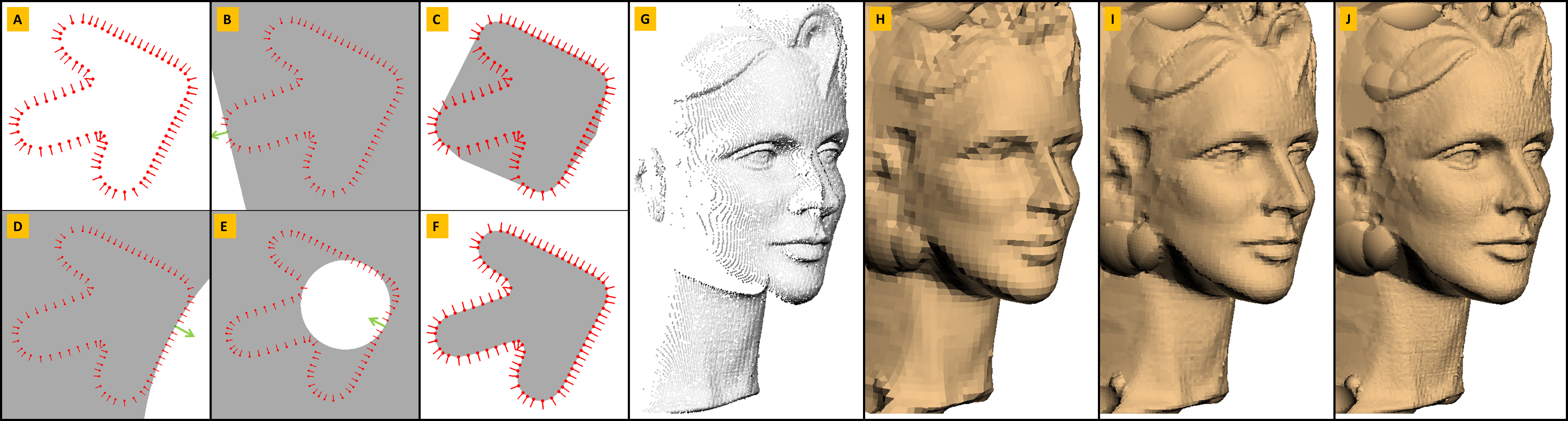 Figure 1 A: A 2D oriented point cloud. B: A supporting
linear half space for one of the oriented points. C: The oriented
convex hull (OCH) of the point cloud. D: An outside supporting circle
for one of the points. E: Inside supporting circles are obtained by
inverting the orientation vectors. F: The non-convex hull (NCH) of
the oriented point cloud is the intersection of the complement of all
the outside supporting circles. G: A 3D oriented point cloud. NCH
surface reconstructions based on octrees of depth 7 (H), 8 (I), and 9
(J).
Figure 1 A: A 2D oriented point cloud. B: A supporting
linear half space for one of the oriented points. C: The oriented
convex hull (OCH) of the point cloud. D: An outside supporting circle
for one of the points. E: Inside supporting circles are obtained by
inverting the orientation vectors. F: The non-convex hull (NCH) of
the oriented point cloud is the intersection of the complement of all
the outside supporting circles. G: A 3D oriented point cloud. NCH
surface reconstructions based on octrees of depth 7 (H), 8 (I), and 9
(J).
In this paper we are concerned with the problem of reconstructing an oriented watertight surface approximating a finite set of points with associated unit length orientation vectors, consistently oriented with respect to the sampled surface \(S\). Oriented point clouds are produced by laser scanners, structured lighting systems, multi-view stereo algorithms, and simulation algorithms.
The prior art on surface reconstruction from point clouds is extensive, spanning more than two decades. Most combinatorial algorithms produce interpolating polygon meshes, and some come with guaranteed reconstruction quality [Bernardini et al. 1999; Amenta et al. 2001; Dey 2007].
Since implicit surfaces are watertight, most approximating surface reconstruction methods produce implicit surfaces, and through variational formulations reduce the problem to the solution of large sparse linear systems [Kazhdan et al. 2006; Alliez et al. 2007; Man- son et al. 2008; Hoppe et al. 1992; Boissonnat and Cazals 2002; Calakli and Taubin 2011; Alexa et al. 2003; Fleishman et al. 2005; Ohtake et al. 2005]. The estimated implicit function is often evaluated on a regular grid of sufficient resolution, and a polygon mesh approximation is generated using an isosurface algorithm such as Marching Cubes [Lorensen and Cline 1987]. Since the cost of estimating or evaluating the implicit function on a regular grid is often excessive, some methods perform the computations on adaptive volumetric meshes such as octrees which require more complex contouring algorithms [Ohtake et al. 2005; Kazhdan et al. 2006; Manson et al. 2008; Calakli and Taubin 2011].
The method proposed in this paper falls somewhere in between these categories. A continuous interpolating piecewise quadratic NCH Signed Distance function is constructed as a function of the oriented point locations and orientation vectors through a simple and direct computation. Then the NCH Signed Distance function is evaluated on the vertices of a volumetric mesh, such as a regular voxel grid or octree constructed as a function of the point locations. Finally an isosurface algorithm is also used to generate an approximating polygonal mesh. When the volumetric mesh is conforming, the polygon mesh is guaranteed to be watertight.
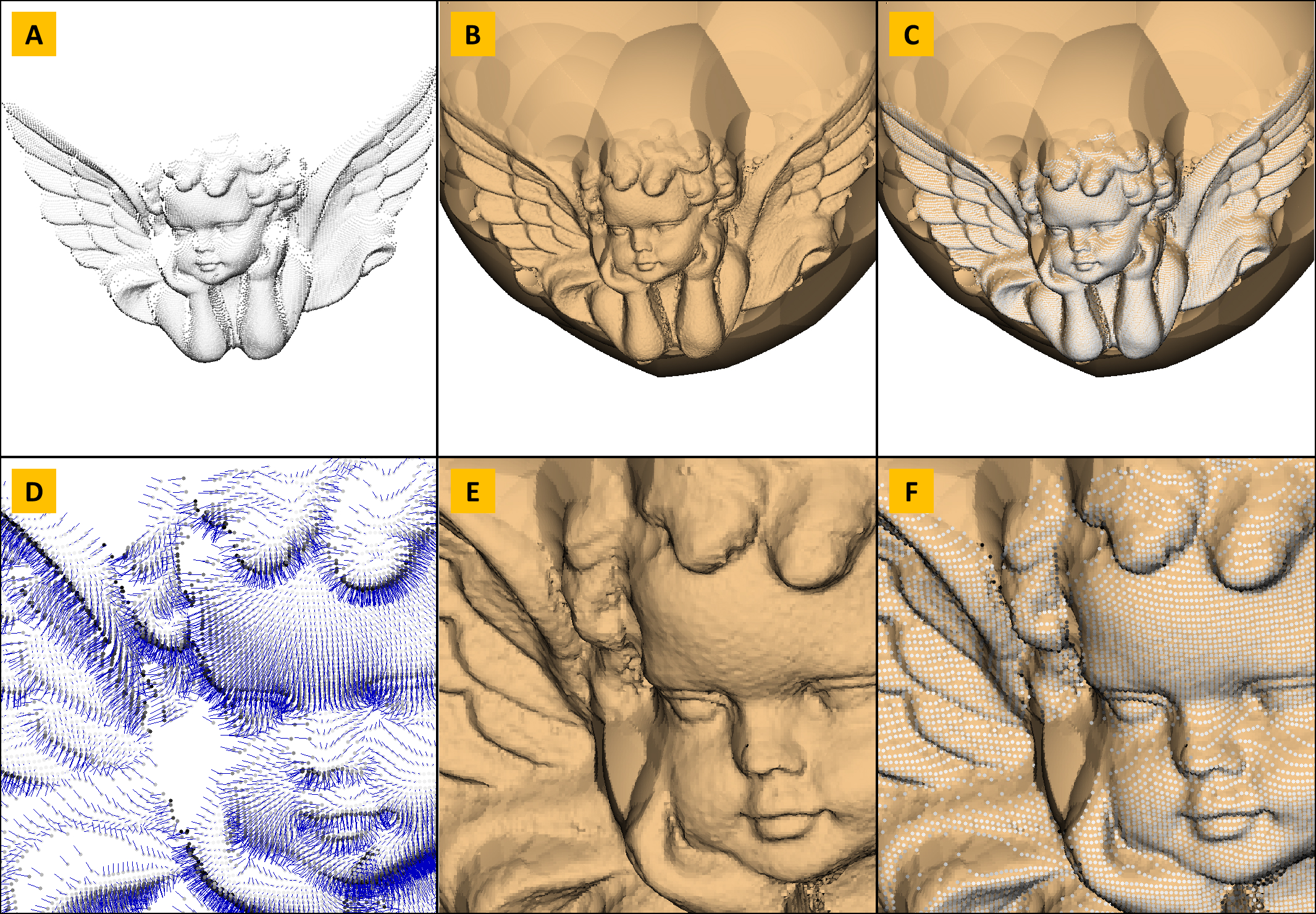 Figure 2 A: An oriented point cloud with approximately 25K
points. B: The polygon mesh extracted by the naive algorithm on a
5003 voxel grid. C: The oriented points superimposed with the mesh.
D: Detail view of the point cloud showing points and orientation
vectors. E: Close-up view of B. Close-up view of C. Note that the
polygon density is higher than the point cloud sampling rate. The
reconstructed polygon mesh has 556,668 vertices and 555,386 faces.
Figure 2 A: An oriented point cloud with approximately 25K
points. B: The polygon mesh extracted by the naive algorithm on a
5003 voxel grid. C: The oriented points superimposed with the mesh.
D: Detail view of the point cloud showing points and orientation
vectors. E: Close-up view of B. Close-up view of C. Note that the
polygon density is higher than the point cloud sampling rate. The
reconstructed polygon mesh has 556,668 vertices and 555,386 faces.
The Naïve Algorithm
To emphasize the simplicity of the proposed method, in this section we describe what we call the Naïve NCH Surface Reconstruction algorithm. In subsequent sections explain why it works, and variations. The Naïve NCH Surface Reconstruction algorithm for a finite set of oriented points comprises three steps: 1) estimating one NCH Signed Distance parameter for each data point; 2) evaluating the NCH Signed Distance function on the vertices of a volumetric mesh such as a regular voxel grid or octree; 3) approximating the zero level set of the NCH Signed Distance function by a polygon mesh using an isosurface algorithm such as Marching Cubes [Lorensen and Cline 1987].
For a finite set of points \({\cal P}=\{ p_1,\ldots,p_N\}\), with associated unit length orientation vectors \(n_1,\ldots,n_N\) we define the value of the NCH Signed Distance function at a 3D point \(x\) as the maximum over \(N\) basis functions,
\begin{equation} f(x) = \max_{1\leq i\leq N} f_i(x) \label{eq:nch-signed-distance-function-finite} \end{equation}where for each oriented point \((p_i,n_i)\), we have one basis function
\begin{equation} f_i(x) = n_i^t(x-p_i)-\rho_i\|x-p_i\|^2 \label{eq:nch-signed-distance-basis-function-finite} \end{equation}The parameter \(\rho_i\) is set equal to zero if the set \(J_i\) of indices \(j=1,\ldots,N\) such that \(n_i^t(p_j-p_i)>0\) is empty, and otherwise
\begin{equation} \rho_i = \min \left\{\frac{n_i^t(p_j-p_i)}{\|p_j-p_i\|^2} : j\in J_i \right\} > 0\;. \label{eq:nch-rho-finite} \end{equation}Figure 2 shows one result obtained with exactly this algorithm.
The main advantage of the Naïve NCH Surface Reconstruction algorithm is its simplicity, since it can be implemented literally with only a few lines of code. The main disadvantage of the method is that its complexity is quadratic in the number of points. We address this issue through an adaptive subsampling approach which yields NCH Surfaces which interpolate only a subset of the input points, and approximates the remaining points under user-specified maximum error.
Even though large areas of missing data points and holes are filled because the output mesh is watertight (except for its intersection with boundaries of the bounding box), the algorithm not always fills holes in an intuitive manner, as can be observed in figure 1. Some of the surface reconstruction algorithms based on variational principles mentioned in the introduction tend to fill holes in a more intuitive and predictable fashion. However, since it is not iterative, this algorithm is robust, and in many cases it can deal gracefully with uneven sampling, as shown in figure 5 .
Non-Convex Hull
In this paper we refer to a half space as a set \(H = \{ x : f(x)\leq 0 \}\) of points satisfying an inequality constraint for a continuous real-valued function \(f(x)\) defined for every point \(x\) in a certain domain \(U\) contained in the ambient space (2D or 3D here). A linear half space is defined by a linear function \(f(x)\). Given a set of points \({\cal P}\), finite or infinite, and not necessarily oriented, the half space \(H\) defined above (with \(f(x)\) linear or non-linear) is said to be a supporting half space for \({\cal P}\) if the following two conditions are satisfied: 1) the set \({\cal P}\) is contained in \(H\), i.e., \({\cal P}\subseteq H\); and 2) there is at least one point \(p\) in \({\cal P}\) where the function attains the value zero \(f(p)=0\). The Convex Hull \(\hbox{CH}({\cal P})\) of the set \({\cal P}\) can be defined as the intersection of all the supporting linear half spaces for \({\cal P}\). Since a linear half space is a convex set, and convexity is preserved by intersection, \(\hbox{CH}({\cal P})\) is also a convex set.
For the finite set of points \(\{ p_1,\ldots,p_N\}\), with associated unit length orientation vectors \(n_1,\ldots,n_N\) we adopt a more restricted definition which takes into account the point orientations. Each oriented point \(p_i\) defines a linear half space \(H_i = \{ x : f_i(x)\leq 0\}\) for the linear function \(f_i(x)=n_i^t(x-p_i)\). We define the Oriented Convex Hull of the set of points \(\hbox{OCH}({\cal P})\) as the intersection of all the supporting linear half spaces \(H_i\). Note that if the orientation of the points is reversed, a completely different result is usually obtained, since the family of supporting linear half spaces is different, and often even empty.
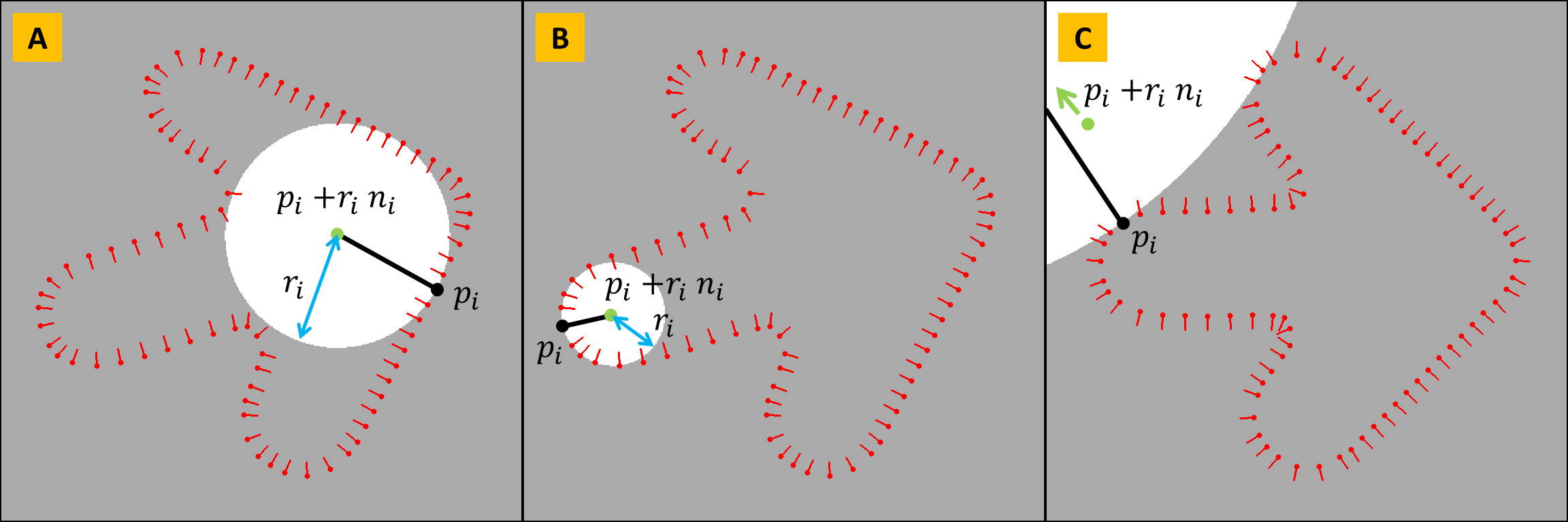 Figure 3
The geometry of the spherical support functions \(f_p(x)\).
Figure 3
The geometry of the spherical support functions \(f_p(x)\).
Since the Oriented Convex Hull is a convex set, it cannot approximate the boundary surface of an object with concavities. To be able to approximate these surfaces we need to augment the family of supporting half spaces. It is necessary for this family to include non-convex half spaces, so that their intersection can represent solid objects with concavities. For each point \(p_i\) in the data set \({\cal P}\) with associated orientation vector \(n_i\), and every positive value of \(r>0\), we consider the function
\begin{equation} f_i^r(x)=\frac{1}{2r}\left\{r^2-\|x-(p_i+r\,n_i)\|^2\right\} \label{eq:spherical-support-function-r} \end{equation}defined for \(x\) in the domain \(U\). This function is positive inside a sphere of radius \(r\) centered at the point \(q=p_i+r\,n_i\), negative outside the sphere, attains its maximum value \(r/2\) at the center point \(q\), and has unit slope \(\|\nabla\!f_i^r(x)\|=1\) at every point \(x\) where\(f_i^r(x)\) is equal to zero.
As shown in figure 3, the point \(q=p_i+r\,n_i\) is located on the ray defined by the point \(p_i\) and vector \(n_i\) at distance \(r\) from \(p_i\). In addition, \(f_i^r(p)=0\), and \(\nabla\!f_i^r(p)=n_i\) for all values of \(r\). Now we define \(r_i\) as the largest value of \(r\) so that \(f_i^r(p_j)\leq 0\) for every other point \(p_j\in{\cal P}\). For finite sets of oriented points we have \(r_i>0\) for each data point \(p_i\in {\cal P}\). As a result, the half space \(H_i\) defined by the function \(f_i(x)=f_i^{r_i}(x)\) of equation \ref{eq:nch-signed-distance-basis-function-finite} is supporting, where \(\rho_i=1/(2r_i)>0\). We refer to these sets \(H_i\) as complementary spherical supporting half spaces. For the linear supporting half spaces to be included as special cases, we need to allow \(\rho_i=0\), or \(r_i=\infty\). Note that, as opposed to the Oriented Convex Hull case, here every oriented point \(p_i\) in the data set has an associated supporting half space \(H_i\), and if the orientations are reversed (\(n_i\mapsto -n_i\)), completely different half spaces are obtained.
The value of \(\rho_i\) for an oriented point \(p_i\) is computed as the minimum over all the positive values
\begin{equation} \rho_{ij} =\frac{n_i^t(p_j-p_i)}{\|p_j-p_i\|^2} \label{eq:rho-ij} \end{equation}over all \(j\neq i\). Note that if \(\rho_{ij}\leq 0\) for all \(j\neq i\), then we should set \(\rho_i=0\), because in this case the linear half space \(H_i=\{x:n_i^t(x-p_i)\}\) is supporting for the set \({\cal P}\).
We define the Non-Convex Hull of the oriented point set \({\cal P}\), denoted \(\hbox{NCH}({\cal P})\), as the intersection of all the complementary spherical supporting half spaces \(H_i\), as defined above. This is the same as saying that the complement of \(\hbox{NCH}({\cal P})\) is a union of balls. Note that \(\hbox{NCH}({\cal P})\) is also a half space. Namely, the half space defined by the continuous signed distance function \(f(x)\) shown in equation \ref{eq:nch-signed-distance-function-finite}. This function is well defined when the data set \({\cal P}\) is bounded, and in particular when it is finite.

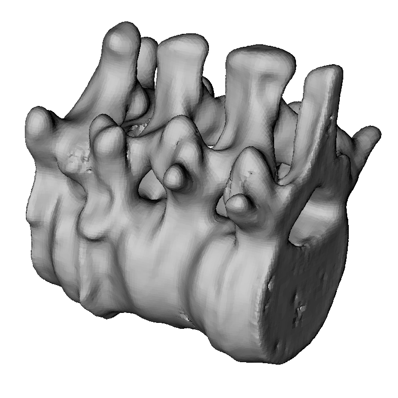
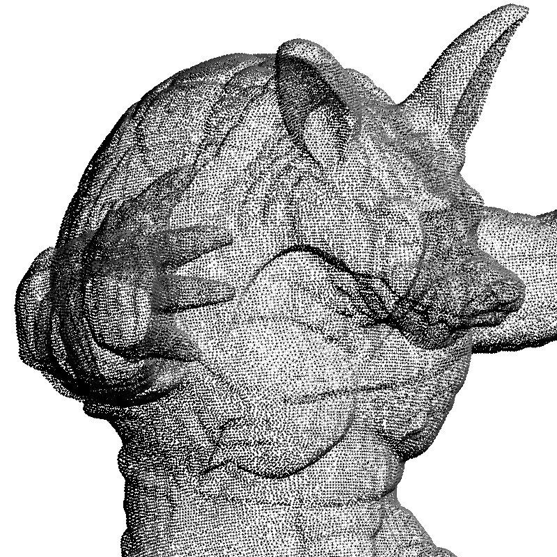

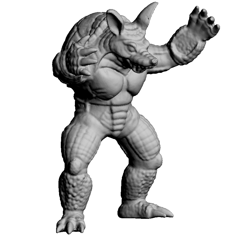
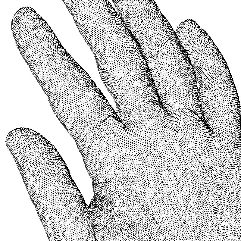
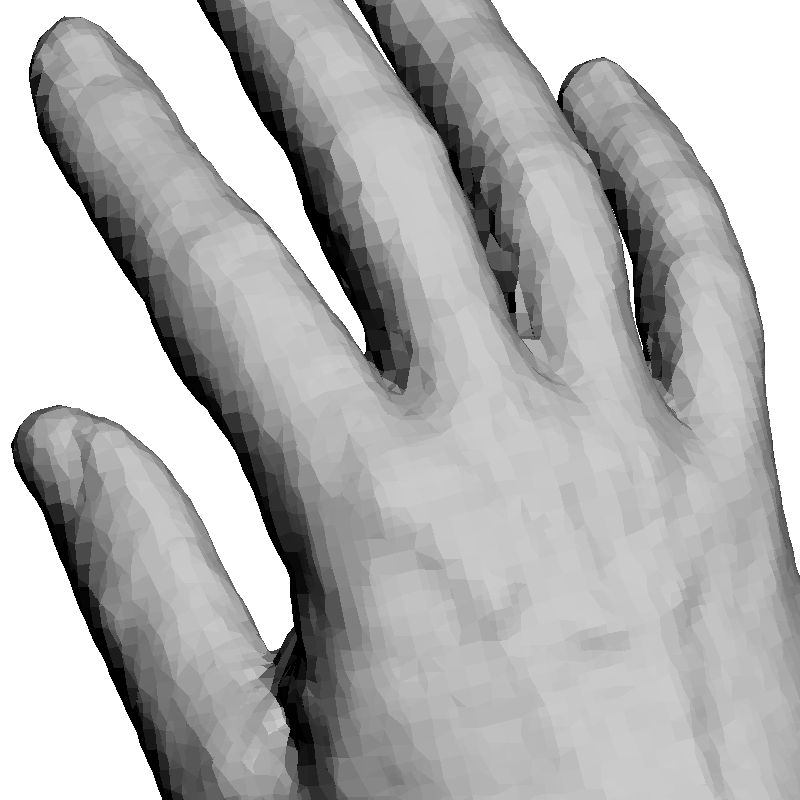
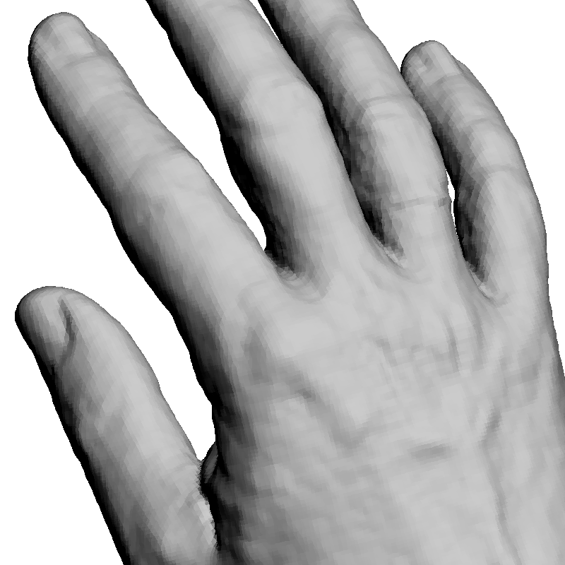
Figure 4
Results on evenly sampled low noise surfaces. Left: Oriented points.
Center: Reconstruction with an octree of depth 9.
Right: Reconstruction with an octree of depth 10.
Relation to the Medial Axis Transform
In this section we assume that the set of points \({\cal P}\) is a sampling of the boundary surface \(S\) of a bounded solid object \(O\), and that the object \(O\) is an open set in 3D. As a result, the surface \(S\) is bounded, orientable (separates the inside from the outside of \(O\)), closed, and it has no boundary (i.e., no holes). Furthermore we assume that it is smooth, has a continuous unit length normal field pointing towards the inside of \(O\), and has continuous curvatures.
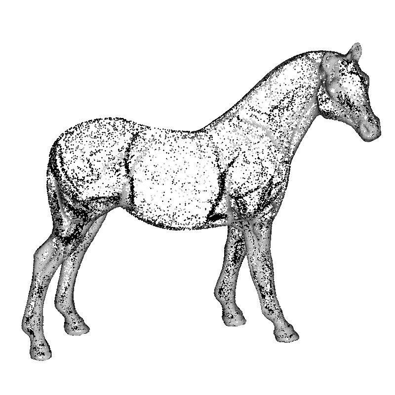
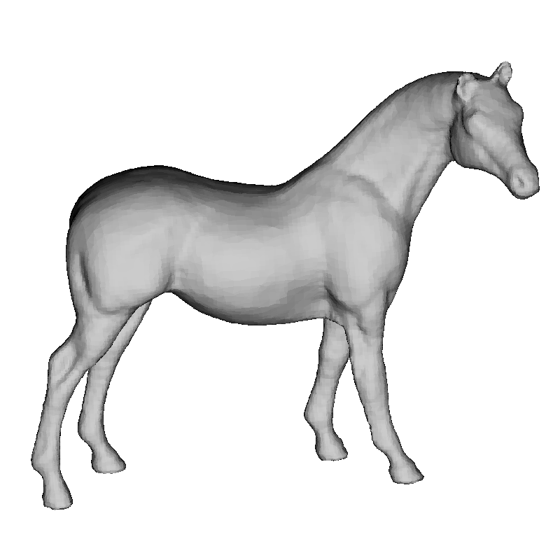

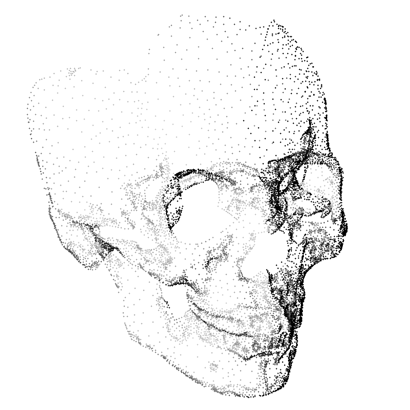
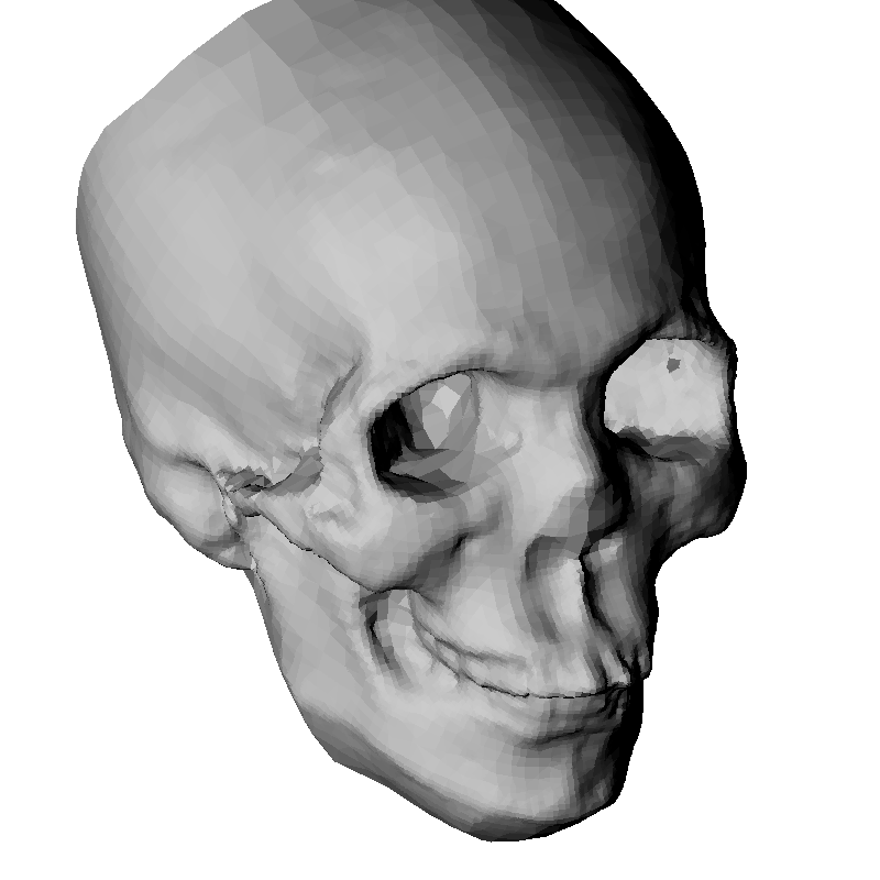

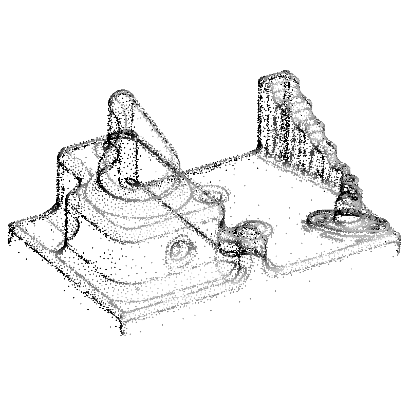
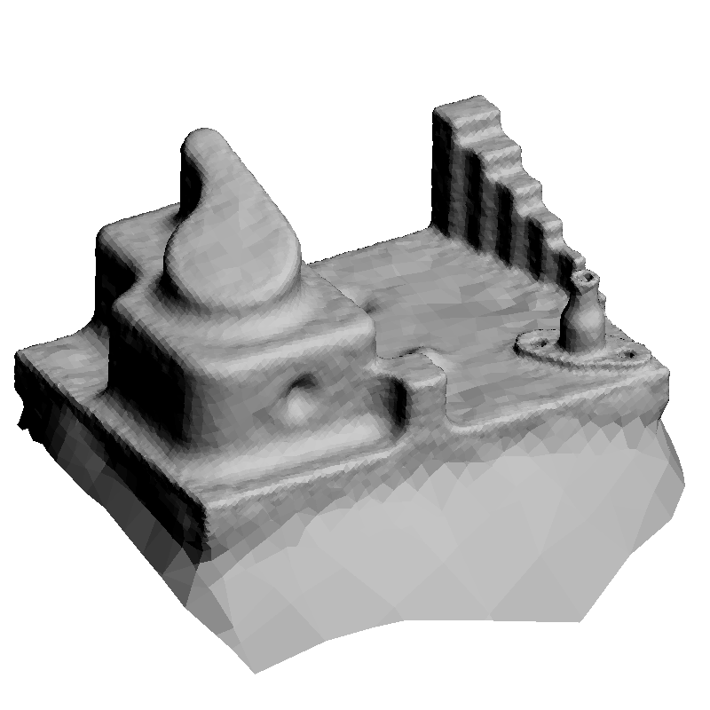
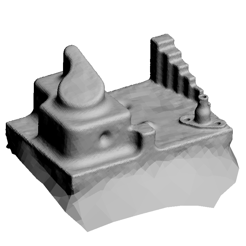
Figure 5
Results on unevenly sampled surfaces. Left: Oriented points.
Center: Reconstruction with an octree of depth 9.
Right: Reconstruction with an octree of depth 10.
The Medial Axis Transform (MAT) is a representation of the object \(O\)
as a union of balls. A ball \(B=B(q,r)=\{x:\|x-q\|
We define the Medial Axis \(\hbox{MA}(O)\) of \(O\) as the set of centers of medial balls. Since two different medial balls cannot have the same center, the mapping \(\hbox{MA}(O)\rightarrow \hbox{MAT}(O)\) which assigns each medial ball center to the corresponding medial ball is well defined, 1-1 and onto. Another way of describing the Medial Axis Transform is as a set of points called Medial Axis Set, augmented with a non-negative radius function which assigns to each medial ball center the corresponding medial ball radius. These radii are, of course, not independent of each other.
In this paper we present an alternative description of the Medial Axis Transform, where each medial ball is not described by its center and radius, but by one of its boundary points and the radius. If \(B\) is a medial ball of center \(q\) and radius \(r\), \(p\) is a point in the intersection of the boundary of \(B\) and \(S\), and \(n_p\) is the surface normal to \(S\) at \(p\) pointing towards the interior of \(O\), since the boundary of \(B\) and \(S\) are tangent, the ball center \(q\) must lie on the normal ray defined by \(p\) and \(n\), in which case we have \(q=p+rn_p\). In addition, because of the maximality of the ball \(B\), the radius \(r\) is uniquely determined: it must be equal to the maximum of radii \(r'>0\) of balls centered at points \(q'=p+r'n\) lying on the ray defined by the point \(p\) and the vector \(n\), fully contained in \(O\). On the other hand, if \(p\) is a point on the surface \(S\), since \(O\) is the union of all the medial balls, and \(S\) is the boundary of this set, a medial ball \(B\) must exists so that \(p\) belongs to the intersection of the boundary of \(B\) and \(S\).
In summary, every medial ball can be written as \(B(p+r_p n_p,r_p)\) for at least one surface point \(p\), where
\begin{equation} r_p = \max \{ r'>0 : B(p+r'n_p,r')\subset O\}\;. \label{eq:nch-continuous-radius} \end{equation} Note that in the mapping \(S\rightarrow \hbox{MAT}(O)\) so defined, two or more surface points may map onto the same medial ball. But this is not a problem, and in fact it is an unusual event; what is important is that every medial ball is accounted for, so that the surface \(S\) can be reconstructed as the boundary of the union of balls \begin{equation} O = \cup \{B(p+r_p n_p,r_p) : p\in S \}\;. \label{eq:S-reconstruction-as union-of-balls} \end{equation}The surface \(S\) can is approximated as the boundary of the Non-Convex Hull \(\hbox{NCH}({\cal P})\) defined as a half space of the NCH Signed Distance \(f(x)\). The Local Feature Size \(\hbox{LFS}(p)\) at a surface point \(p\in S\) is usually defined as the distance from \(p\) to the nearest point in the Symmetric Medial Axis [Amenta et al. 2001; Dey 2007]. A finite set \({\cal P}\subset S\) is defined as an \(\epsilon\)-sample of \(S\) if the distance from any point \(p\in S\) to its closest sample in \({\cal P}\) is at most \(\epsilon\,\hbox{LFS}(p)\). Several authors have shown that for sufficiently small \(\epsilon\) the surface reconstructed as the boundary of \(\hbox{MAT}({\cal P})\) is a geometrically accurate approximation of \(S\) [Amenta et al. 2001; Dey 2007], and our experiments validate these theoretical results.
Octrees and Isosurfaces
Since typically the NCH Signed Distance function has constant sign in large regions, one way to potentially reduce the computational cost of the naïve algorithm is to detect those areas and not to evaluate the function there. Following a standard recursive space partition approach, we build an octree as a function of the point locations and the orientation vectors, we evaluate the NCH Signed Distance function at the vertices of the volumetric mesh, and use the Dual Marching Cubes (MC) algorithm [Schaefer and Warren 2005] to generate an output polygon mesh. Since the dual mesh of an octree is a conforming volumetric polyhedral mesh, the polygon meshes produced by DMC are adaptive, but have no cracks. The results shown in figures 4 and 5 have been computed using our implementation of DMC. Although the results presented are very good, we regard them as preliminary work. Due to lack of space, the details of this process as well as extensive experimental results will be presented in a future extended publication.
Conclusion
We have introduced an extremely simple algorithm to reconstruct watertight surfaces from finite sets of oriented points. The formulation generalizes the Convex Hull in such a way that concavities can be represented and approximated. We have also proposed preliminary strategies to reduce the computational cost by generating adaptive polygon meshes and by subsampling. Despite its simplicity, the proposed algorithm produces high quality polygon meshes competitive with those produced by state-of-the-art algorithms. Since the algorithm is massively paralellizable, and we plan to produce a GPU implementation in the near future.
Acknowledgements
This material is based upon work supported by the National Science Foundation under grants CCF-0729126, IIS-0808718, CCF-0915661, and IIP-1215308.
References
ALEXA, M., BEHR, J., COHEN-OR, D., FLEISHMAN, S., LEVIN, D., AND SILVA, C. 2003. Computing and rendering point set surfaces. IEEE Transactions on Visualization and Computer Graphics, 3–15.
ALLIEZ, P., COHEN-STEINER, D., TONG, Y., AND DESBRUN, M. 2007. Voronoi-based variational reconstruction of unoriented point sets. In Proceedings of the fifth Eurographics symposium on Geometry processing, Eurographics Association, 39–48.
AMENTA, N., CHOI, S., AND KOLLURI, R. 2001. The Power Crust, Unions of Balls, and the Medial Axis Transform. Computational Geometry Theory and Applications 19, 2-3 (jul), 127– 153.
BERNARDINI, F., MITTLEMAN, J., RUSHMEIER, H., SILVA, C., AND TAUBIN, G. 1999. The Ball-Pivoting Algorithm for Surface Reconstruction. IEEE Transactions on Visualization and Computer Graphics 5, 4, 349–359.
BOISSONNAT, J., AND CAZALS, F. 2002. Smooth surface reconstruction via natural neighbour interpolation of distance functions. Computational Geometry 22, 1, 185–203.
CALAKLI, F., AND TAUBIN, G. 2011. SSD: Smooth Signed Distance Surface Reconstruction. Computer Graphics Forum 30, 7. http://mesh.brown.edu/ssd.
DEY, T. 2007. Curve and surface reconstruction: algorithms with mathematical analysis. Cambridge University Press.
FLEISHMAN, S., COHEN-OR, D., AND SILVA, C. T. 2005. Robust moving least-squares fitting with sharp features. ACM Transactions on Graphics 24 (July), 544–552.
HOPPE, H., DEROSE, T., DUCHAMP, T., MCDONALD, J., AND STUETZLE, W. 1992. Surface Reconstruction from Unorganized Points. In Proceedings of ACM Siggraph, Citeseer.
KAZHDAN, M., BOLITHO, M., AND HOPPE, H. 2006. Poisson surface reconstruction. In Proceedings of the fourth Eurographics symposium on Geometry processing, Eurographics Association, 61–70.
LORENSEN, W., AND CLINE, H. 1987. Marching Cubes: A High Resolution 3d Surface Construction Algorithm. 163–169.
MANSON, J., PETROVA, G., AND SCHAEFER, S. 2008. Streaming surface reconstruction using wavelets. In Computer Graphics Forum, vol. 27, Wiley Online Library, 1411–1420.
OHTAKE, Y., BELYAEV, A., ALEXA, M., TURK, G., AND SEIDEL, H. 2005. Multi-level partition of unity implicits. In ACM SIGGRAPH 2005 Courses, ACM, 173.
SCHAEFER, S., AND WARREN, J. 2005. Dual Marching Cubes: primal contouring of dual grids. In Computer Graphics Forum, vol. 24, Wiley Online Library, 195–201.