The Mathematics of Optical Triangulation
This course is primarily concerned with the estimation of 3D shape by illuminating the world with certain known patterns, and observing the illuminated objects with cameras. In this chapter we derive models describing this image formation process, leading to the development of reconstruction equations allowing the recovery of 3D shape by geometric triangulation.
We start by introducing the basic concepts in a coordinate-free fashion, using elementary algebra and the language of analytic geometry (e.g., points, vectors, lines, rays, and planes). Coordinates are introduced later, along with relative coordinate systems, to quantify the process of image formation in cameras and projectors.
Perspective Projection and the Pinhole Model
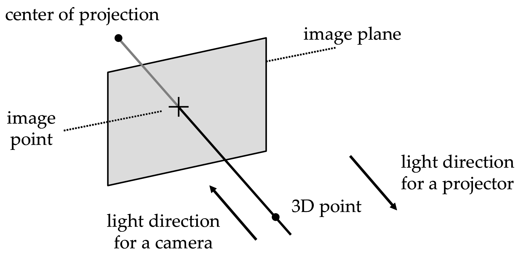
Figure 2.1 Perspective projection under the pinhole model.
A simple and popular geometric model for a camera or a projector is the pinhole model, composed of a plane and a point external to the plane (see Figure 2.1). We refer to the plane as the image plane, and to the point as the center of projection. In a camera, every 3D point (other than the center of projection) determines a unique line passing through the center of projection. If this line is not parallel to the image plane, then it must intersect the image plane in a single image point. In mathematics, this mapping from 3D points to 2D image points is referred to as a perspective projection. Except for the fact that light traverses this line in the opposite direction, the geometry of a projector can be described with the same model. That is, given a 2D image point in the projector's image plane, there must exist a unique line containing this point and the center of projection (since the center of projection cannot belong to the image plane). In summary, light travels away from a projector (or towards a camera) along the line connecting the 3D scene point with its 2D perspective projection onto the image plane.
Geometric Representations
Since light moves along straight lines (in a homogeneous medium such as air), we derive 3D reconstruction equations from geometric constructions involving the intersection of lines and planes, or the approximate intersection of pairs of lines (two lines in 3D may not intersect). Our derivations only draw upon elementary algebra and analytic geometry in 3D (e.g., we operate on points, vectors, lines, rays, and planes). We use lower case letters to denote points \(p\) and vectors \(v\). All the vectors will be taken as column vectors with real-valued coordinates \(v\in\mathbb{R}^3\), which we can also regard as matrices with three rows and one column \(v\in\mathbb{R}^{3\times 1}\). The length of a vector \(v\) is a scalar \(\|v\|\in\mathbb{R}\). We use matrix multiplication notation for the inner product \(v_1^tv_2\in\mathbb{R}\) of two vectors \(v_1\) and \(v_2\), which is also a scalar. Here \(v_1^t\in\mathbb{R}^{1\times 3}\) is a row vector, or a \(1\times 3\) matrix, resulting from transposing the column vector \(v_1\). The value of the inner product of the two vectors \(v_1\) and \(v_2\) is equal to \(\|v_1\|\|v_2\|\cos(\alpha)\), where \(\alpha\) is the angle formed by the two vectors ( \(0\leq\alpha\leq 180^{\circ}\)). The \(3\times N\) matrix resulting from concatenating \(N\) vectors \(v_1,\ldots,v_N\) as columns is denoted \([v_1|\cdots|v_N]\in\mathbb{R}^{3\times N}\). The vector product \(v_1\times v_2\in\mathbb{R}^3\) of the two vectors \(v_1\) and \(v_2\) is a vector perpendicular to both \(v_1\) and \(v_2\), of length \(\|v_1\times v_2\|=\|v_1\|\,\|v_2\|\,\sin(\alpha)\), and direction determined by the right hand rule (i.e., such that the determinant of the matrix \([v_1|v_2|v_1\times v_2]\) is non-negative). In particular, two vectors \(v_1\) and \(v_2\) are linearly dependent ( i.e., one is a scalar multiple of the other), if and only if the vector product \(v_1\times v_2\) is equal to zero.Points and Vectors
Since vectors form a vector space, they can be multiplied by scalars and added to each other. Points, on the other hand, do not form a vector space. But vectors and points are related: a point plus a vector \(p+v\) is another point, and the difference between two points \(q-p\) is a vector. If \(p\) is a point, \(\lambda\) is a scalar, and \(v\) is a vector, then \(q=p+\lambda v\) is another point. In this expression, \(\lambda v\) is a vector of length \(|\lambda|\,\|v\|\). Multiplying a point by a scalar \(\lambda p\) is not defined, but an affine combination of \(N\) points \(\lambda_1 p_1+\cdots+\lambda_N p_N\), with \(\lambda_1+\cdots+\lambda_N=1\), is well defined:
\begin{equation} \lambda_1 p_1+\cdots+\lambda_Np_N = p_1+\lambda_2(p_2-p_1)+\cdots+\lambda_N(p_N-p_1)\;. \end{equation}
Parametric Representation of Lines and Rays
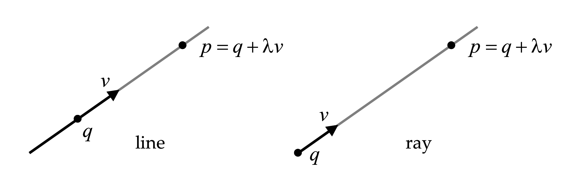
Figure 2.2 Parametric representation of lines and rays.
A line \(L\) can be described by specifying one of its points \(q\) and a direction vector \(v\) (see Figure 2.2). Any other point \(p\) on the line \(L\) can be described as the result of adding a scalar multiple \(\lambda v\), of the direction vector \(v\), to the point \(q\) ( \(\lambda\) can be positive, negative, or zero): \begin{equation} L = \{\; p=q+\lambda v\;:\;\lambda\in\mathbb{R}\;\}\;. \label{eq:line-parametric} \end{equation} This is the parametric representation of a line, where the scalar \(\lambda\) is the parameter. Note that this representation is not unique, since \(q\) can be replaced by any other point on the line \(L\), and \(v\) can be replaced by any non-zero scalar multiple of \(v\). However, for each choice of \(q\) and \(v\), the correspondence between parameters \(\lambda\in\mathbb{R}\) and points \(p\) on the line \(L\) is one-to-one.
A ray is half of a line . While in a line the parameter \(\lambda\) can take any value, in a ray it is only allowed to take non-negative values. \[ R = \{\; p=q+\lambda v \;:\;\lambda\geq 0\;\} \] In this case, if the point \(q\) is changed, a different ray results. Since it is unique, the point \(q\) is called the origin of the ray. The direction vector \(v\) can be replaced by any positive scalar multiple, but not by a negative scalar multiple. Replacing the direction vector \(v\) by a negative scalar multiple results in the opposite ray. By convention in projectors, light traverses rays along the direction determined by the direction vector. Conversely in cameras, light traverses rays in the direction opposite to the direction vector (i.e., in the direction of decreasing \(\lambda\)).
Parametric Representation of Planes
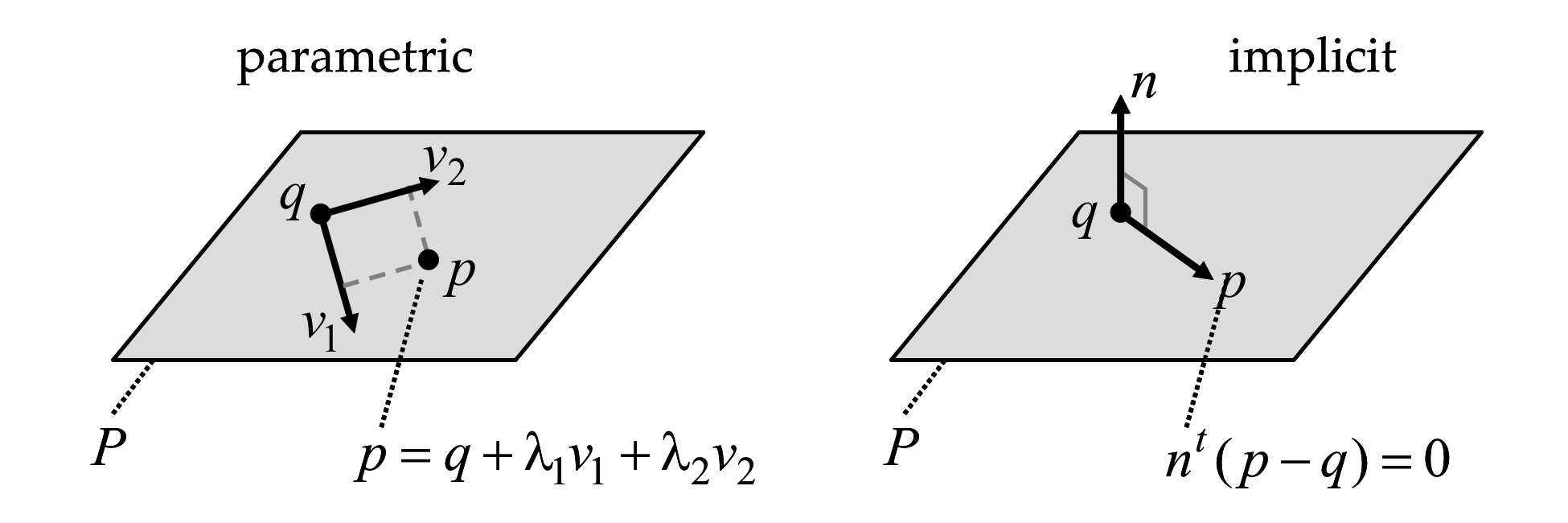
Figure 2.3 Parametric and implicit representations of planes.
Similar to how lines are represented in parametric form, a plane \(P\) can be described in parametric form by specifying one of its points \(q\) and two linearly independent direction vectors \(v_1\) and \(v_2\) (see Figure 2.3. Any other point \(p\) on the plane \(P\) can be described as the result of adding scalar multiples \(\lambda_1 v_1\) and \(\lambda_2 v_2\) of the two vectors to the point \(q\), as follows. \[ P = \{\; p=q+\lambda_1 v_1 + \lambda_2 v_2 \;:\;\lambda_1,\lambda_2\in\mathbb{R}\;\} \] As in the case of lines, this representation is not unique. The point \(q\) can be replaced by any other point in the plane, and the vectors \(v_1\) and \(v_2\) can be replaced by any other two linearly independent linear combinations of \(v_1\) and \(v_2\).
Implicit Representation of Planes
A plane \(P\) can also be described in implicit form as the set of zeros of a linear equation in three variables. Geometrically, the plane can be described by one of its points \(q\) and a normal vector \(n\). A point \(p\) belongs to the plane \(P\) if and only if the vectors \(p-q\) and \(n\) are orthogonal:
\begin{equation} P = \{\; p\;:\: n^t(p-q)=0 \;\}\;. \label{eq:plane-implicit} \end{equation}
Again, this representation is not unique. The point \(q\) can be replaced by any other point in the plane, and the normal vector \(n\) by any non-zero scalar multiple \(\lambda n\).
To convert from the parametric to the implicit representation, we can take the normal vector \(n=v_1\times v_2\) as the vector product of the two basis vectors \(v_1\) and \(v_2\). To convert from implicit to parametric, we need to find two linearly independent vectors \(v_1\) and \(v_2\) orthogonal to the normal vector \(n\). In fact, it is sufficient to find one vector \(v_1\) orthogonal to \(n\). The second vector can be defined as \(v_2=n\times v_1\). In both cases, the same point \(q\) from one representation can be used in the other.
Implicit Representation of Lines
A line \(L\) can also be described in implicit form as the intersection of two planes, both represented in implicit form, such that \begin{equation} L = \{\; p\;:\; n_1^t(p-q)=n_2^t(p-q)=0 \;\}, \label{eq:line-implicit} \end{equation} where the two normal vectors \(n_1\) and \(n_2\) are linearly independent (if \(n_1\) an \(n_2\) are linearly dependent, rather than a line, the two equations describe the same plane). Note that when \(n_1\) and \(n_2\) are linearly independent, the two implicit representations for the planes can be defined with respect to a common point belonging to both planes, rather than to two different points. Since a line can be described as the intersection of many different pairs of planes, this representation is not unique. The point \(q\) can be replaced by any other point belonging to the intersection of the two planes, and the two normal vectors can be replaced by any other pair of linearly independent linear combinations of the two vectors.
To convert from the parametric representation of Equation \ref{eq:line-parametric} to the implicit representation of Equation \ref{eq:line-implicit}, one needs to find two linearly independent vectors \(n_1\) and \(n_2\) orthogonal to the direction vector \(v\). One way to do so is to first find one non-zero vector \(n_1\) orthogonal to \(v\), and then take \(n_2\) as the vector product \(n_2=v\times n_1\) of \(v\) and \(n_1\). To convert from implicit to parametric, one needs to find a non-zero vector \(v\) orthogonal to both normal vectors \(n_1\) and \(n_2\). The vector product \(v=n_1\times n_2\) is one such vector, and any other is a scalar multiple of it.
Reconstruction by Triangulation
It is common for projected illumination patterns used in laser scanning and structured lighting to contain identifiable lines or points. Under the pinhole projector model, a projected line creates a plane of light (the unique plane containing the line on the image plane and the center of projection), and a projected point creates a ray of light (the unique line containing the image point and the center of projection).
While the intersection of a ray of light with the object being scanned can be considered as a single illuminated point, the intersection of a plane of light with the object generally contains many illuminated curved segments. Each of these segments is composed of many illuminated points. A single illuminated point, visible to the camera, defines a camera ray. For now, we assume that the locations and orientations of projector and camera are known with respect to the global coordinate system (with procedures for estimating these quantities covered in the Chapter on Camera and Projector Calibration ). Under this assumption, the equations of projected planes and rays, as well as the equations of camera rays corresponding to illuminated points, are defined by parameters which can be measured. From these measurements, the location of illuminated points can be recovered by intersecting the planes or rays of light with the camera rays corresponding to the illuminated points. Through such procedures the depth ambiguity introduced by pinhole projection can be eliminated, allowing recovery of a 3D surface model.
Line-Plane Intersection
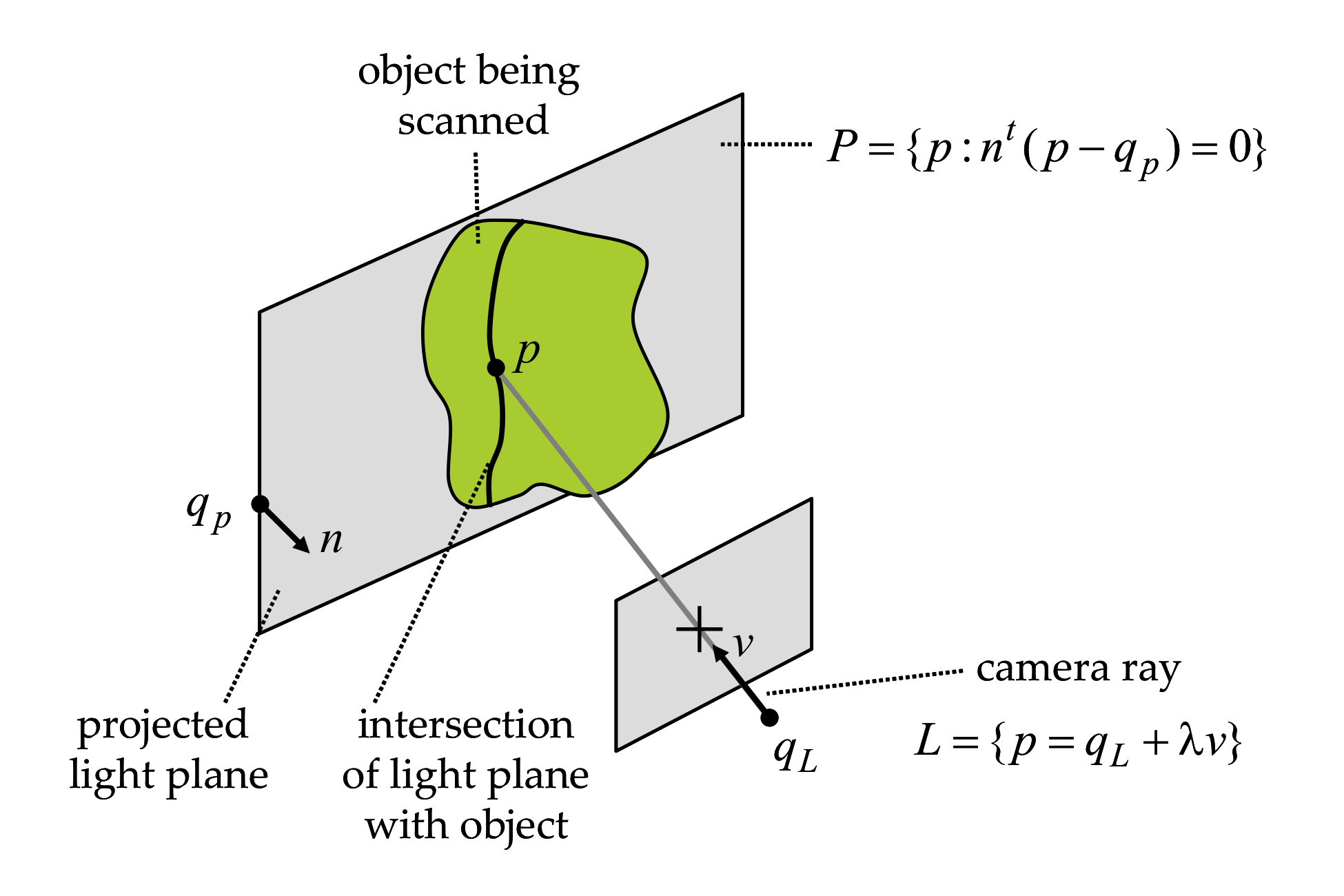
Figure 2.4 Triangulation by line-plane intersection.
Computing the intersection of a line and a plane is straightforward when the line is represented in parametric form \[ L = \{\; p=q_L+\lambda v \;:\;\lambda\in\mathbb{R}\;\}, \] and the plane is represented in implicit form \[ P = \{\; p\;:\: n^t(p-q_P)=0 \;\}\;. \] Note that the line and the plane may not intersect, in which case we say that the line and the plane are parallel. This is the case if the vectors \(v\) and \(n\) are orthogonal \(n^tv=0\). The vectors \(v\) and \(n\) are also orthogonal when the line \(L\) is contained in the plane \(P\). Whether or not the point \(q_L\) belongs to the plane \(P\) differentiates one case from the other. If the vectors \(v\) and \(n\) are not orthogonal \(n^tv\neq 0\), then the intersection of the line and the plane contains exactly one point \(p\). Since this point belongs to the line, it can be written as \(p=q_L+\lambda v\), for a value \(\lambda\) which we need to determine. Since the point also belongs to the plane, the value \(\lambda\) must satisfy the linear equation \[ n^t(p-q_p)= n^t(\lambda v + q_L-q_p)=0\;, \] or equivalently \begin{equation} \lambda = \frac{n^t(q_P-q_L)}{n^tv}\;. \label{eq:lambda-line-plane-intersection} \end{equation} Since we have assumed that the line and the plane are not parallel (i.e., by checking that \(n^tv\neq 0\) beforehand), this expression is well defined. A geometric interpretation of line-plane intersection is provided in Figure 2.4.
Line-Line Intersection
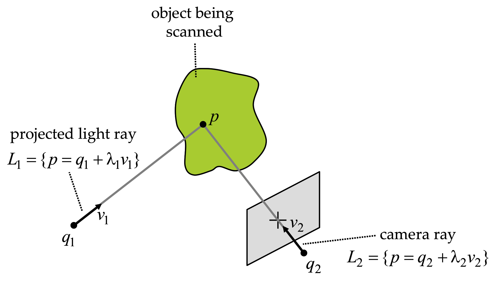
Figure 2.5 Triangulation by line-line intersection.
We consider here the intersection of two arbitrary lines \(L_1\) and \(L_2\), as shown in Figure 2.5. \[ L_1=\{\; p=q_1+\lambda_1 v_1\;:\;\lambda_1\in\mathbb{R}\} \quad \hbox{and} \quad L_2=\{ p=q_2+\lambda_2 v_2\;:\;\lambda_2\in\mathbb{R}\;\} \]
Let us first identify the special cases. The vectors \(v_1\) and \(v_2\) can be linearly dependent (i.e., if one is a scalar multiple of the other) or linearly independent.
The two lines are parallel if the vectors \(v_1\) and \(v_2\) are linearly dependent. If, in addition, the vector \(q_2-q_1\) can also be written as a scalar multiple of \(v_1\) or \(v_2\), then the lines are identical. Of course, if the lines are parallel but not identical, they do not intersect.
If \(v_1\) and \(v_2\) are linearly independent, the two lines may or may not intersect. If the two lines intersect, the intersection contains a single point. The necessary and sufficient condition for two lines to intersect, when \(v_1\) and \(v_2\) are linearly independent, is that scalar values \(\lambda_1\) and \(\lambda_2\) exist so that \[ q_1+\lambda_1 v_1 = q_2+\lambda_2 v_2, \] or equivalently so that the vector \(q_2-q_1\) is linearly dependent on \(v_1\) and \(v_2\).
Since two lines may not intersect, we define the approximate intersection as the point which is closest to the two lines. More precisely, whether two lines intersect or not, we define the approximate intersection as the point \(p\) which minimizes the sum of the square distances to both lines \( \phi(p,\lambda_1,\lambda_2)=\|q_1+\lambda_1 v_1-p\|^2+\|q_2+\lambda_2 v_2-p\|^2\;.\) As before, we assume \(v_1\) and \(v_2\) are linearly independent, such the approximate intersection is a unique point.
To prove that the previous statement is true, and to determine the value of \(p\), we follow an algebraic approach. The function \(\phi(p,\lambda_1,\lambda_2)\) is a quadratic non-negative definite function of five variables, the three coordinates of the point \(p\) and the two scalars \(\lambda_1\) and \(\lambda_2\).
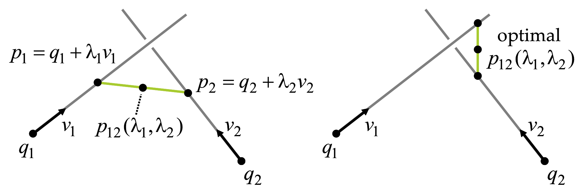
Figure 2.6 Parametric and implicit representations of planes.
We first reduce the problem to the minimization of a different quadratic non-negative definite function of only two variables \(\lambda_1\) and \(\lambda_2\). Let \(p_1=q_1+\lambda_1 v_1\) be a point on the line \(L_1\), and let \(p_2=q_2+\lambda_2 v_2\) be a point on the line \(L_2\). Define the midpoint \(p_{12}\), of the line segment joining \(p1\) and \(p2\), as \[ p_{12}=p_1+\frac{1}{2}(p_2-p_1)=p_2+\frac{1}{2}(p_1-p_2)\;. \] A necessary condition for the minimizer \((p,\lambda_1,\lambda_2)\) of \(\phi\) is that the partial derivatives of \(\phi\), with respect to the five variables, all vanish at the minimizer. In particular, the three derivatives with respect to the coordinates of the point \(p\) must vanish \[ \frac{\partial\phi}{\partial p} = (p-p_1)+(p-p_2) = 0\;, \] or equivalently, it is necessary for the minimizer point \(p\) to be the midpoint \(p_{12}\) of the segment joining \(p_1\) and \(p_2\) (see Figure 2.6).
As a result, the problem reduces to the minimization of the square distance from a point \(p_1\) on line \(L_1\) to a point \(p_2\) on line \(L_2\). Practically, we must now minimize the quadratic non-negative definite function of two variables \[ \psi(\lambda_1,\lambda_2)= 2\phi(p_{12},\lambda_1,\lambda_2)=\|(q_2+\lambda_2v_2)-(q_1+\lambda_1v_1)\|^2\;. \] Note that it is still necessary for the two partial derivatives of \(\psi\), with respect to \(\lambda_1\) and \(\lambda_2\), to be equal to zero at the minimum, as follows. \[ \frac{\partial \psi}{\partial\lambda_1} = v_1^t(\lambda_1 v_1-\lambda_2 v_2+q_1-q_2) = \lambda_1 \|v_1\|^2-\lambda_2 v_1^tv_2+v_1^t(q_1-q_2) = 0 \] \[ \frac{\partial \psi}{\partial\lambda_2} = v_2^t(\lambda_2 v_2-\lambda_1 v_1+q_2-q_1) = \lambda_2 \|v_2\|^2-\lambda_2 v_2^tv_1+v_2^t(q_2-q_1) = 0 \] These provide two linear equations in \(\lambda_1\) and \(\lambda_2\), which can be concisely expressed in matrix form as \[ \left(\begin{matrix} \|v_1\|^2 & -v_1^tv_2 \cr -v_2^tv_1 & \|v_2\|^2 \end{matrix}\right) \left(\begin{matrix} \lambda_1 \cr \lambda_2 \end{matrix}\right) = \left(\begin{matrix} v_1^t(q_2-q_1) \cr v_2^t(q_1-q_2) \end{matrix}\right)\;. \] It follows from the linear independence of \(v_1\) and \(v_2\) that the \(2\times 2\) matrix on the left hand side is non-singular. As a result, the unique solution to the linear system is given by \[ \left(\begin{matrix} \lambda_1 \cr \lambda_2 \end{matrix}\right) = \left(\begin{matrix} \|v_1\|^2 & -v_1^tv_2 \cr -v_2^tv_1 & \|v_2\|^2 \end{matrix}\right)^{-1} \left(\begin{matrix} v_1^t(q_2-q_1) \cr v_2^t(q_1-q_2) \end{matrix}\right) \] or equivalently \begin{equation} \left(\begin{matrix} \lambda_1 \cr \lambda_2 \end{matrix}\right) = \frac{1}{ \|v_1\|^2\|v_2\|^2-(v_1^tv_2)^2 } \left(\begin{matrix} \|v_2\|^2 & v_1^tv_2 \cr v_2^tv_1 & \|v_1\|^2 \end{matrix}\right) \left(\begin{matrix} v_1^t(q_2-q_1) \cr v_2^t(q_1-q_2) \end{matrix}\right)\;. \label{eq:lambda-line-line-intersection} \end{equation} In conclusion, the approximate intersection \(p\) can be obtained from the value of either \(\lambda_1\) or \(\lambda_2\) provided by these expressions.
Coordinate Systems
So far we have presented a coordinate-free description of triangulation. In practice, however, image measurements are recorded in discrete pixel units. In this section we incorporate such coordinates into our prior equations, as well as document the various coordinate systems involved.
Image Coordinates and the Pinhole Camera
Consider a pinhole model with camera coordinate sytem comprising a center of projection \(q\), and orthonormal basis \(\{v_1,v_2,v_3\}\), and image plane spanned by the first two basis vectros at focal length \(f=1\). Any 3D point \(p\), not necessarily on the image plane, has coordinates \((p^1,p^2,p^3)^t\) relative to the camera coordinate system. The projection of the point \(p\) onto the image plane is a 2D image point defined by the parameters \(u^1\) and \(u^2\), which can be written as a 3D vector \(u=(u^1,u^2,1)\). Using this notation the point \(p\) is expressed as \[ \left( \begin{matrix} p^1\cr p^2\cr p^3 \end{matrix} \right) = \lambda \, \left( \begin{matrix} u^1\cr u^2\cr 1 \end{matrix} \right) \] where \(\lambda\) is a non-negative parameter.
The Ideal Pinhole Camera
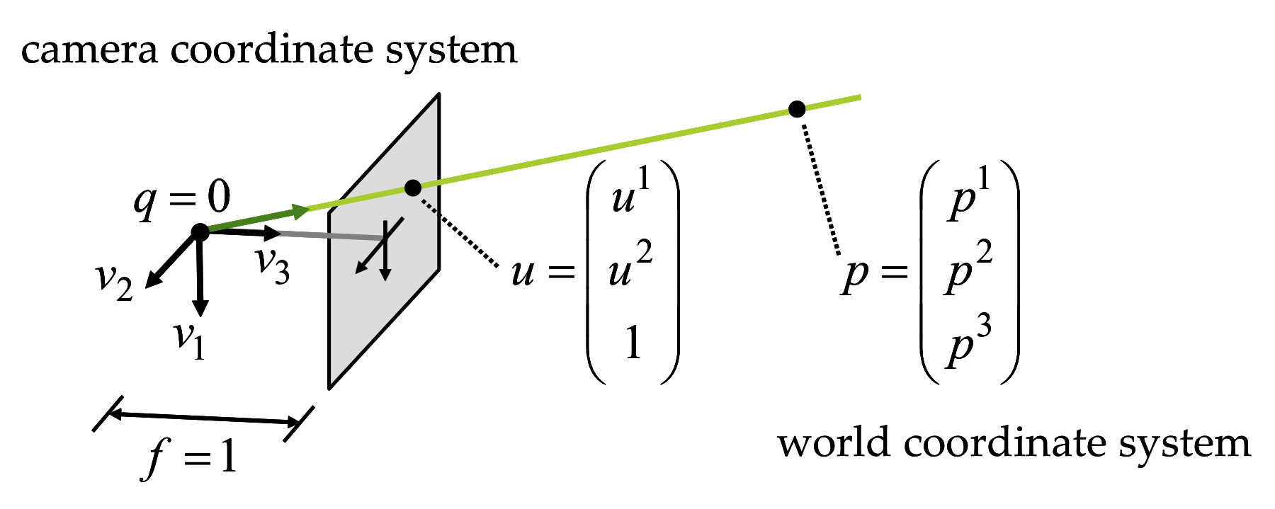
Figure 2.7 The ideal pinhole camera.
In the ideal pinhole camera shown in Figure 2.7, the center of projection \(o\) is at the origin of the world coordinate system, with coordinates \((0,0,0)^t\), and the point \(q\) and the vectors \(v_1\) and \(v_2\) are defined as \[ [v_1|v_2|q]= \left( \begin{matrix} 1&0&0\cr 0&1&0\cr 0&0&1 \end{matrix} \right)\;. \] Note that not every 3D point has a projection on the image plane. Points without a projection are contained in a plane parallel to the image passing through the center of projection. An arbitrary 3D point \(p\) with coordinates \((p^1,p^2,p^3)^t\) belongs to this plane if \(p^3=0\), otherwise it projects onto an image point with the following coordinates. \[ \begin{matrix} u^1 & = & p^1/p^3\cr u^2 & = & p^2/p^3 \end{matrix} \] There are other descriptions for the relation between the coordinates of a point and the image coordinates of its projection; for example, the projection of a 3D point \(p\) with coordinates \((p^1,p^2,p^3)^t\) has image coordinates \(u=(u^1,u^2,1)\) if, for some scalar \(\lambda\neq 0\), we can write
\begin{equation} \lambda\; \left( \begin{matrix} u^1\cr u^2\cr 1 \end{matrix} \right) = \left( \begin{matrix} p^1\cr p^2\cr p^3 \end{matrix} \right)\;. \label{eq:ideal-pinhole-projection} \end{equation}
The General Pinhole Camera
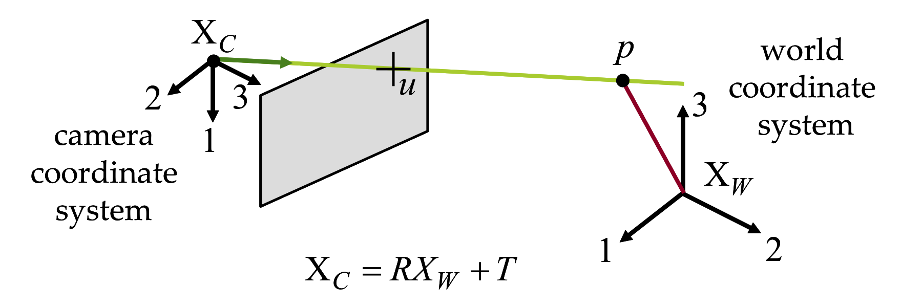
Figure 2.8 The general pinhole model.
The center of a general pinhole camera is not necessarily placed at the origin of the world coordinate system and may be arbitrarily oriented. However, it does have a camera coordinate system attached to the camera, in addition to the world coordinate system (see Figure 2.8). A 3D point \(p\) has world coordinates described by the vector \(p_W=(p_W^1,p_W^2,p_W^3)^t\) and camera coordinates described by the vector \(p_C=(p_C^1,p_C^2,p_C^3)^t\). These two vectors are related by a rigid body transformation specified by a translation vector \(T\in\mathbb{R}^3\) and a rotation matrix \(R\in\mathbb{R}^{3\times 3}\), such that \[ p_C=R\,p_W+T\;. \] In camera coordinates, the relation between the 3D point coordinates and the 2D image coordinates of the projection is described by the ideal pinhole camera projection (i.e., Equation \ref{eq:ideal-pinhole-projection}), with \(\lambda u = p_C\). In world coordinates this relation becomes \begin{equation} \lambda\,u = R\,p_W\,+\,T\;. \label{eq:general-pinhole-projection} \end{equation} The parameters \((R,T)\), which are referred to as the extrinsic parameters of the camera, describe the location and orientation of the camera with respect to the world coordinate system.
Equation \ref{eq:general-pinhole-projection} assumes that the unit of measurement of lengths on the image plane is the same as for world coordinates, that the distance from the center of projection to the image plane is equal to one unit of length, and that the origin of the image coordinate system has image coordinates \(u^1=0\) and \(u^2=0\). None of these assumptions hold in practice. For example, lengths on the image plane are measured in pixel units, and in meters or inches for world coordinates, the distance from the center of projection to the image plane can be arbitrary, and the origin of the image coordinates is usually on the upper left corner of the image. In addition, the image plane may be tilted with respect to the ideal image plane. To compensate for these limitations of the current model, a matrix \(K\in\mathbb{R}^{3\times 3}\) is introduced in the projection equations to describe intrinsic parameters as follows. \begin{equation} \lambda\,u = K(R\,p_W\,+\,T) \label{eq:general-pinhole-projection-with-intrinsic} \end{equation} The matrix \(K\) has the following form \[ K= \left( \begin{matrix} f\,s_1 & f\,s_\theta & o^1 \cr 0 & f\,s_2 & o^2 \cr 0 & 0 & 1 \end{matrix} \right)\;, \] where \(f\) is the focal length (i.e., the distance between the center of projection and the image plane). The parameters \(s_1\) and \(s_2\) are the first and second coordinate scale parameters, respectively. Note that such scale parameters are required since some cameras have non-square pixels. The parameter \(s_\theta\) is used to compensate for a tilted image plane. Finally, \((o^1,o^2)^t\) are the image coordinates of the intersection of the vertical line in camera coordinates with the image plane. This point is called the image center or principal point. Note that all intrinsic parameters embodied in \(K\) are independent of the camera pose. They describe physical properties related to the mechanical and optical design of the camera. Since in general they do not change, the matrix \(K\) can be estimated once through a calibration procedure and stored (as will be described in the following chapter). Afterwards, image plane measurements in pixel units can immediately be ``normalized'', by multiplying the measured image coordinate vector by \(K^{-1}\), so that the relation between a 3D point in world coordinates and 2D image coordinates is described by Equation \ref{eq:general-pinhole-projection}.
Real cameras also display non-linear lens distortion, which is also considered intrinsic. Lens distortion compensation must be performed prior to the normalization described above. We will discuss appropriate lens distortion models in Chapter Calibration.
Lines from Image Points
As shown in Figure 2.4, an image point with coordinates \(u=(u^1,u^2,1)^t\) defines a unique line containing this point and the center of projection. The challenge is to find the parametric equation of this line, as \(L=\{p=q+\lambda\,v\,:\,\lambda\in\mathbb{R}\}\). Since this line must contain the center of projection, the projection of all the points it spans must have the same image coordinates. If \(p_W\) is the vector of world coordinates for a point contained in this line, then world coordinates and image coordinates are related by Equation \ref{eq:general-pinhole-projection} such that \(\lambda\,u = R\,p_W\,+\,T\). Since \(R\) is a rotation matrix, we have \(R^{-1}=R^t\) and we can rewrite the projection equation as \[ p_W = (-R^tT)+\lambda\,(R^tu)\;. \] In conclusion, the line we are looking for is described by the point \(q\) with world coordinates \(q_W=-R^tT\), which is the center of projection, and the vector \(v\) with world coordinates \(v_W=R^tu\).
Planes from Image Lines
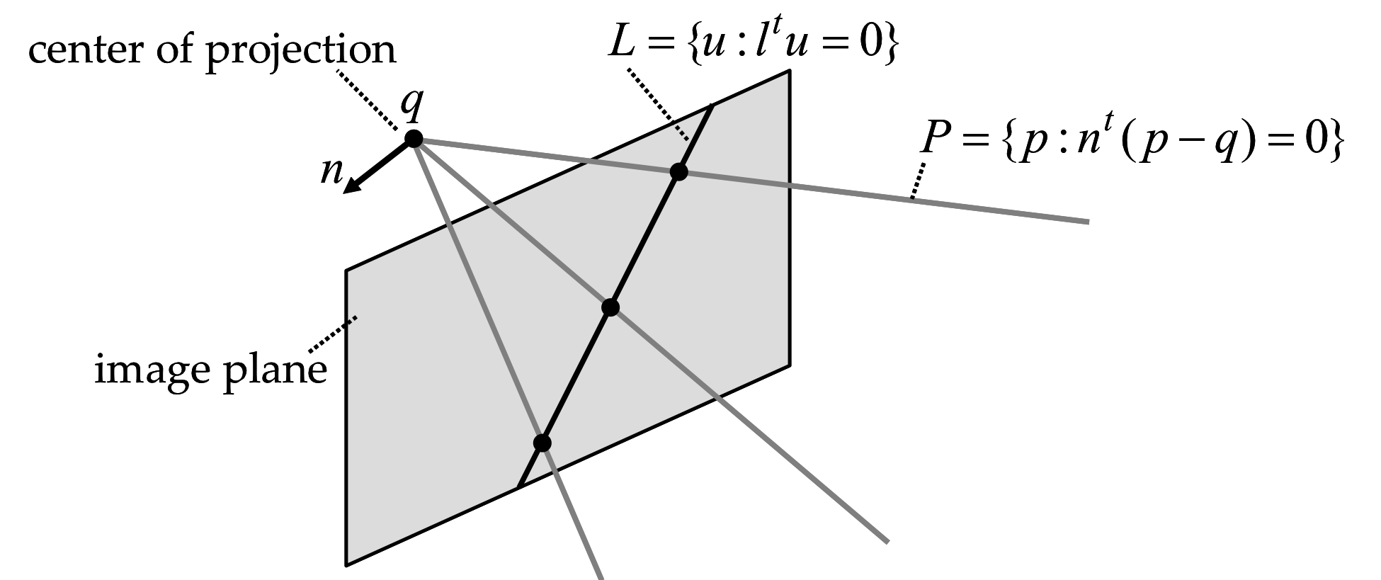
Figure 2.9 The plane defined by an image line and the center of projection.
A straight line on the image plane can be described in either parametric or implicit form, both expressed in image coordinates. Let us first consider the implicit case. A line on the image plane is described by one implicit equation of the image coordinates \[ L=\{u:l^tu=l^1u^1+l^2u^2+l^3=0\}\;, \] where \(l=(l^1,l^2,l^3)^t\) is a vector with \(l^1\neq 0\) or \(l^2\neq 0\). Using active illumination, projector patterns containing vertical and horizontal lines are common. Thus, the implicit equation of an horizontal line is \[ L_H=\{u:l^tu=u^2-\nu=0\}\;, \] where \(\nu\) is the second coordinate of a point on the line. In this case we can take \(l=(0,1,-\nu)^t\). Similarly, the implicit equation of a vertical line is \[ L_V=\{u:l^tu=u^1-\nu=0\}\;, \] where \(\nu\) is now the first coordinate of a point on the line. In this case we can take \(l=(1,0,-\nu)^t\). There is a unique plane \(P\) containing this line \(L\) and the center of projection. For each image point with image coordinates \(u\) on the line \(L\), the line containing this point and the center of projection is contained in \(P\). Let \(p\) be a point on the plane \(P\) with world coordinates \(p_W\) projecting onto an image point with image coordinates \(u\). Since these two vectors of coordinates satisfy Equation \ref{eq:general-pinhole-projection}, for which \(\lambda\,u = R\,p_W\,+\,T\), and the vector \(u\) satisfies the implicit equation defining the line \(L\), we have \[ 0 = \lambda l^tu = l^t(R\,p_W\,+\,T)= (R^tl)^t\,(p_W - (-R^tT))\;. \] In conclusion, the implicit representation of plane \(P\), corresponding to Equation \ref{eq:plane-implicit} for which \(P=\{p:n^t(p-q)=0\}\), can be obtained with \(n\) being the vector with world coordinates \(n_W=R^tl\) and \(q\) the point with world coordinates \(q_W=-R^tT\), which is the center of projection.