Reconstructing Surfaces From Point Clouds
The objects scanned in the previous examples are solid, with a well-defined boundary surface separating the inside from the outside. Since computers have a finite amount of memory and operations need to be completed in a finite number of steps, algorithms can only be designed to manipulate surfaces described by a finite number of parameters. Perhaps the simplest surface representation with a finite number of parameters is produced by a finite sampling scheme, where a process systematically chooses a set of points lying on the surface.
The triangulation-based 3D scanners described in previous chapters produce such a finite sampling scheme. The so-called point cloud, a dense collection of surface samples, has become a popular representation in computer graphics. However, since point clouds do not constitute surfaces, they cannot be used to determine which 3D points are inside or outside of the solid object. For many applications, being able to make such a determination is critical. For example, without closed bounded surfaces, volumes cannot be measured. Therefore, it is important to construct so-called watertight surfaces from point clouds. In this chapter we consider these issues.
Representation and Visualization of Point Clouds
In addition to the 3D point locations, the 3D scanning methods described in previous chapters are often able to estimate a color per point, as well as a surface normal vector. Some methods are able to measure both color and surface normal, and some are able to estimate other parameters which can be used to describe more complex material properties used to generate complex renderings. In all these cases the data structure used to represent a point cloud in memory is a simple array. A minimum of three values per point are needed to represent the point locations. Colors may require one to three more values per point, and normals vectors three additional values per point. Other properties may require more values, but in general it is the same number of parameters per point that need to be stored. If \(M\) is the number of parameters per point and \(N\) is the number of points, then point cloud can be represented in memory using an array of length \(NM\).
File Formats
Storing and retrieving arrays from files is relatively simple, and storing the raw data either in ASCII format or in binary format is a valid solution to the problem. However, these solutions may be incompatible with many software packages. We want to mention two standards which have support for storing point clouds with some auxiliary attributes.
Storing Point Clouds as VRML Files
The Virtual Reality Modeling Language (VRML) is an ISO standard
published in 1997. A VRML file describes a scene graph comprising a
variety of nodes. Among geometry nodes, PointSet and IndexedFaceSet are used to store point clouds. The
PointSet node was designed to
store point clouds, but in addition to the 3D coordinates of each
point, only colors can be stored. No other attributes can be stored in
this node. In particular, normal vectors cannot be recorded. This is a
significant limitation, since normal vectors are important both for
rendering point clouds and for reconstructing watertight surfaces from
point clouds.
The IndexedFaceSet node was
designed to store polygon meshes with colors, normals, and/or texture
coordinates. In addition to vertex coordinates, colors and normal
vectors can be stored bound to vertices. Even though
the IndexedFaceSet node was not
designed to represent point clouds, the standard allows for this node
to have vertex coordinates and properties such as colors and/or
normals per vertex, but no faces. The standard does not specify how
such a node should be rendered in a VRML browser, but since they
constitute valid VRML files, they can be used to store point clouds.
The SFL File Format
The SFL file format was introduced with
Pointshop3D [ZPKG02] to provide
a versatile file format to import and export point clouds with color,
normal vectors, and a radius per vertex describing the local sampling
density. A SFL file is encoded in binary and features an extensible
set of surfel attributes, data compression, upward and downward
compatibility, and transparent conversion of surfel attributes,
coordinate systems, and color spaces. Pointshop3D is a software
system for interactive editing of point-based surfaces, developed at
the Computer Graphics Lab at ETH Zurich.
Visualization
A well-established technique to render dense point clouds is point splatting. Each point is regarded as an oriented disk in 3D, with the orientation determined by the surface normal evaluated at each point, and the radius of the disk usually stored as an additional parameter per vertex. As a result, each point is rendered as an ellipse. The color is determined by the color stored with the point, the direction of the normal vector, and the illumination model. The radii are chosen so that the ellipses overlap, resulting in the perception of a continuous surface being rendered.
Merging Point Clouds
The triangulation-based 3D scanning methods described in previous chapters are able to produce dense point clouds. However, due to visibility constraints these point clouds may have large gaps without samples. In order for a surface point to be reconstructed, it has to be illuminated by a projector, and visible by a camera. In addition, the projected patterns needs to illuminate the surface transversely for the camera to be able to capture a sufficient amount of reflected light. In particular, only points on the front-facing side of the object can be reconstructed (i.e., on the same side as the projector and camera). Some methods to overcome these limitations are discussed in the Conclusion. However, to produce a complete representation, multiple scans taken from various points of view must be integrated to produce a point cloud with sufficient sampling density over the whole visible surface of the object being scanned.
Computing Rigid Body Matching Transformations
The main challenge to merging multiple scans is that each scan is produced with respect to a different coordinate system. As a result, the rigid body transformation needed to register one scan with another must be estimated. In some cases the object is moved with respect to the scanner under computer control. In those cases the transformations needed to register the scans are known within a certain level of accuracy. This is the case when the object is placed on a computer-controlled turntable or linear translation stage. However, when the object is repositioned by hand, the matching transformations are not known and need to be estimated from point correspondences.
We now consider the problem of computing the rigid body transformation \(q=Rp+T\) to align two shapes from two sets of \(N\) points, \(\{p_1,\ldots,p_N\}\) and \(\{q_1,\ldots,q_N\}\). That is, we are looking for a rotation matrix \(R\) and a translation vector \(T\) so that
\[ q_1=Rp_1+T\quad\ldots\quad q_N=Rp_N+T\;. \]The two sets of points can be chosen interactively or automatically. In either case, being able to compute the matching transformation in closed form is a fundamental operation.
This registration problem is, in general, not solvable due to measurement errors. A common approach in such a case is to seek a least-squares solution. In this case, we desire a closed-form solution for minimizing the mean squared error
\begin{equation} \phi(R,T)=\frac{1}{N}\sum_{i=1}^N \|Rp_i+T-q_i\|^2\;, \label{eq:matching-error-RT} \end{equation}over all rotation matrices \(R\) and translation vectors \(T\). This yields a quadratic function of 12 components in \(R\) and \(T\); however, since \(R\) is restricted to be a valid rotation matrix, there exist additional constraints on \(R\). Since the variable \(T\) is unconstrained, a closed-form solution for \(T\), as a function of \(R\), can be found by solving the linear system of equations resulting from differentiating the previous expression with respect to \(T\).
\[ \frac{1}{2}\frac{\partial\phi}{\partial T} = \frac{1}{N}\sum_{i=1}^N (Rp_i+T-q_i) = 0 \Rightarrow T= \overline{q}-R\overline{p} \]In this expression \(\overline{p}\) and \(\overline{q}\) are the geometric centroids of the two sets of matching points, given by
\[ \overline{p}=\left(\frac{1}{N}\sum_{i=1}^Np_i\right)\qquad \overline{q}=\left(\frac{1}{N}\sum_{i=1}^Nq_i\right)\;. \]Substituting for \(T\) in Equation \ref{eq:matching-error-RT}, we obtain the following equivalent error function which depends only on \(R\).
\begin{equation} \psi(R)=\frac{1}{N}\sum_{i=1}^N \|R(p_i-\overline{p})-(q_i-\overline{q})\|^2 \label{eq:matching-error-R} \end{equation}If we expand this expression we obtain
\[ \psi(R)= \frac{1}{N}\sum_{i=1}^N \|p_i-\overline{p}\|^2 -\frac{2}{N}\sum_{i=1}^N (q_i-\overline{q})^tR(p_i-\overline{p}) +\frac{1}{N}\sum_{i=1}^N \|q_i-\overline{q}\|^2\;, \]since \(\|Rv\|^2=\|v\|^2\) for any vector \(v\). As the first and last terms do not depend on \(R\), maximizing this expression is equivalent to maximizing
\[ \eta(R)=\frac{1}{N}\sum_{i=1}^N (q_i-\overline{q})^tR(p_i-\overline{p}) = \hbox{trace}(RM)\;, \]where \(M\) is the \(3\times 3\) matrix
\[ M = \frac{1}{N}\sum_{i=1}^N (p_i-\overline{p})(q_i-\overline{q})^t\;. \]Recall that, for any pair of matrices \(A\) and \(B\) of the same dimensions, \(\hbox{trace}(A^tB)=\hbox{trace}(BA^t)\). We now consider the singular value decomposition (SVD) \(M=U\Delta V^t\), where \(U\) and \(V\) are orthogonal \(3\times 3\) matrices, and \(\Delta\) is a diagonal \(3\times 3\) matrix with elements \(\delta_1\geq\delta_2\geq\delta_3\geq 0\). Substituting, we find
\[ \hbox{trace}(RM)= \hbox{trace}(RU\Delta V^t)= \hbox{trace}((V^tRU)\Delta)= \hbox{trace}(W\Delta)\;, \]where \(W=V^tRU\) is orthogonal. If we expand this expression, we obtain
\[ \hbox{trace}(W\Delta)=w_{11}\delta_1+w_{22}\delta_2+w_{33}\delta_3 \leq\delta_1+\delta_2+\delta_3\;, \]where \(W=(w_{ij})\). The last inequality is true because the components of an orthogonal matrix cannot be larger than one. Note that the last inequality is an equality only if \(w_{11}=w_{22}=w_{33}=1\), which is only the case when \(W=I\) (the identity matrix). It follows that if \(V^tU\) is a rotation matrix, then \(R=V^tU\) is the minimizer of our original problem. The matrix \(V^tU\) is an orthogonal matrix, but it may not have a negative determinant. In that case, an upper bound for \(\hbox{trace}(W\Delta)\), with \(W\) restricted to have a negative determinant, is achieved for \(W=J\), where
\[ J=\left( \begin{matrix} 1 & 0 & 0 \cr 0 & 1 & 0 \cr 0 & 0 & -1 \end{matrix} \right)\;. \]In this case it follows that the solution to our problem is \(R=V^tJU\).
The Iterative Closest Point (ICP) Algorithm
The Iterative Closest Point (ICP) is an algorithm employed to match two surface representations, such as points clouds or polygon meshes. This matching algorithm is used to reconstruct 3D surfaces by registering and merging multiple scans. The algorithm is straightforward and can be implemented in real-time. ICP iteratively estimates the transformation (i.e., translation and rotation) between two geometric data sets. The algorithm takes as input two data sets, an initial estimate for the transformation, and an additional criterion for stopping the iterations. The output is an improved estimate of the matching transformation. The algorithm comprises the following steps:
- Select points from the first shape.
- Associate points, by nearest neighbor, with those in the second shape.
- Estimate the closed-form matching transformation using the method derived in the previous section.
- Transform the points using the estimated parameters.
- Repeat previous steps until the stopping criterion is met.
The algorithm can be generalized to solve the problem of registering multiple scans. Each scan has an associated rigid body transformation which will register it with respect to the rest of the scans, regarded as a single rigid object. An additional external loop must be added to the previous steps to pick one transformation to be optimized with each pass, while the others are kept constant---either going through each of the scans in sequence, or randomizing the choice.
Surface Reconstruction from Point Clouds
Watertight surfaces partition space into two disconnected regions so that every line segment joining a point in one region to a point in the other must cross the dividing surface. In this section we discuss methods to reconstruct watertight surfaces from point clouds.
Continuous Surfaces
In mathematics surfaces are represented in parametric or implicit form. A parametric surface \(S=\{x(u):u\in U\}\) is defined by a function \(x:U\rightarrow\mathbb{R}^3\) on an open subset \(U\) of the plane. An implicit surface is defined as a level set \(S=\{p\in\mathbb{R}^3:f(p)=\lambda\}\) of a continuous function \(f:V\rightarrow\mathbb{R}\), where \(V\) is an open subset in 3D. These functions are most often smooth or piecewise smooth. Implicit surfaces are called watertight because they partition space into the two disconnected sets of points, one where \(f(p)>\lambda\) and a second where \(f(p)<\lambda\). Since the function \(f\) is continuous, every line segment joining a point in one region to a point in the other must cross the dividing surface. When the boundary surface of a solid object is described by an implicit equation, one of these two sets describes the inside of the object, and the other one the outside. Since the implicit function can be evaluated at any point in 3D space, it is also referred to as a scalar field. On the other hand, parametric surfaces may or may not be watertight. In general, it is difficult to determine whether a parametric surface is watertight or not. In addition, implicit surfaces are preferred in many applications, such as reverse engineering and interactive shape design, because they bound a solid object which can be manufactured; for example, using rapid prototyping technologies or numerically-controlled machine tools, such representations can define objects of arbitrary topology. As a result, we focus our remaining discussion on implicit surfaces.
Discrete Surfaces
A discrete surface is defined by a finite number of parameters. We
only consider here polygon meshes, and in particular those polygon
meshes representable as IndexedFaceSet nodes in VRML files. Polygon meshes are
composed of geometry and topological
connectivity. The geometry includes vertex coordinates,
normal vectors, and colors (and possibly texture coordinates). The
connectivity is represented in various ways. A popular representation
used in many isosurface algorithms is the polygon soup, where
polygon faces are represented as loops of vertex coordinate
vectors. If two or more faces share a vertex, the vertex coordinates
are repeated as many times as needed. Another popular representation
used in isosurface algorithms is the \texttt{IndexedFaceSet} (IFS),
describing polygon meshes with simply-connected faces. In this
representation the geometry is stored as arrays of floating point
numbers. In these notes we are primarily concerned with the array
\texttt{coord} of vertex coordinates, and to a lesser degree with the
array \texttt{normal} of face normals. The connectivity is described
by the total number \(V\) of vertices, and \(F\) faces, which are
stored in the \texttt{coordIndex} array as a sequence of loops of
vertex indices, demarcated by values of \(-1\).
Isosurfaces
An isosurface is a polygonal mesh surface representation produced by
an isosurface algorithm. An isosurface algorithm constructs a
polygonal mesh approximation of a smooth implicit surface
\(S=\{x:f(x)= 0\}\) within a bounded three-dimensional volume, from
samples of a defining function \(f(x)\) evaluated on the vertices of a
volumetric grid. Marching Cubes
[LC87]
and related algorithms
operate on function values provided at the vertices of hexahedral
grids. Another family of isosurface algorithms operate on functions
evaluated at the vertices of tetrahedral grids
[DK91]
. Usually, no additional information about the function is
provided, and various interpolation schemes are used to evaluate the
function within grid cells, if necessary. The most natural
interpolation scheme for tetrahedral meshes is linear interpolation,
which we also adopt here.
Isosurface Construction Algorithms
An isosurface algorithm producing a polygon soup output must solve three key problems: (1) determining the quantity and location of isosurface vertices within each cell, (2) determining how these vertices are connected forming isosurface faces, and (3) determining globally consistent face orientations. For isosurface algorithms producing IFS output, there is a fourth problem to solve: identifying isosurface vertices lying on vertices and edges of the volumetric grid. For many visualization applications, the polygon soup representation is sufficient and acceptable, despite the storage overhead. Isosurface vertices lying on vertices and edges of the volumetric grid are independently generated multiple times. The main advantage of this approach is that it is highly parallelizable. But, since most of these boundary vertices are represented at least twice, it is not a compact representation.
Researchers have proposed various solutions and design decisions (e.g., cell types, adaptive grids, topological complexity, interpolant order) to address these four problems. The well-known Marching Cubes (MC) algorithm uses a fixed hexahedral grid (i.e., cube cells) with linear interpolation to find zero-crossings along the edges of the grid. These are the vertices of the isosurface mesh. Second, polygonal faces are added connecting these vertices using a table. The crucial observation made with MC is that the possible connectivity of triangles in a cell can be computed independently of the function samples and stored in a table. Out-of-core extensions, where sequential layers of the volume are processed one at a time, are straightforward.
Similar tetrahedral-based
algorithms
[DK91][GH95][TPG99],
dubbed Marching Tetrahedra (MT), have also been developed (again using
linear interpolation). Although the cell is simpler, MT requires
maintaining a tetrahedral sampling grid. Out-of-core extensions
require presorted traversal schemes, such as in
[CS97].
For an unsorted
tetrahedral grid, hash tables are used to save and retrieve vertices
lying on edges of the volumetric grid. As an example of an isosurface
algorithm, we discuss MT in more detail.
| 0 | 0000 | [-1] |
| 1 | 0001 | [2,1,0,-1] |
| 2 | 0010 | [0,3,4,-1] |
| 3 | 0011 | [1,3,4,2,-1] |
| 4 | 0100 | [1,5,3,-1] |
| 5 | 0101 | [0,2,5,3,-1] |
| 6 | 0110 | [0,3,5,4,-1] |
| 7 | 0111 | [1,5,2,-1] |
| 8 | 1000 | [2,5,1,-1] |
| 9 | 1001 | [4,5,3,0,-1] |
| 10 | 1010 | [3,5,2,0,-1] |
| 11 | 1011 | [3,5,1,-1] |
| 12 | 1100 | [2,4,3,1,-1] |
| 13 | 1101 | [4,3,0,-1] |
| 14 | 1110 | [0,1,2,-1] |
| 15 | 1111 | [-1] |
| 0 | (0,1) |
| 1 | (0,2) |
| 2 | (0,3) |
| 3 | (1,2) |
| 4 | (1,3) |
| 5 | (2,3) |
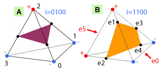
Table 6.1 Look-up tables for tetrahedral mesh isosurface evaluation. Note that consistent face orientation is encoded within the table. Indices stored in the first table reference tetrahedron edges, as indicated by the second table of vertex pairs (and further illustrated in Figure 6.1 ). In this case, only edge indices \(\{1,2,3,4\}\) have associated isosurface vertex coordinates, which are shared with neighboring cells.
Marching Tetrahedra
MT operates on the following input data: (1) a tetrahedral grid and (2) one piecewise linear function \(f(x)\), defined by its values at the grid vertices. Within the tetrahedron with vertices \(x_0,x_1,x_2,x_3\in\mathbb{R}^3\), the function is linear and can be described in terms of the barycentric coordinates \(b=(b_0,b_1,b_2,b_3)^t\) of an arbitrary internal point \(x = b_0\,x_0+b_1\,x_1+b_2\,x_2+b_3\,x_3\) with respect to the four vertices: \(f(x)=b_0\,f(x_0)+b_1\,f(x_1)+b_2\,f(x_2)+b_3\,f(x_3)\), where \(b_0,b_1,b_2,b_3\geq 0\) and \(b_0+b_1+b_2+b_3=1\). As illustrated in Figure 6.1 , the sign of the function at the four grid vertices determines the connectivity (e.g., triangle, quadrilateral, or empty) of the output polygonal mesh within each tetrahedron. There are actually \(16=2^4\) cases, which modulo symmetries and sign changes reduce to only three. Each grid edge, whose end vertex values change sign, corresponds to an isosurface mesh vertex. The exact location of the vertex along the edge is determined by linear interpolation from the actual function values, but note that the \(16\) cases can be precomputed and stored in a table indexed by a 4-bit integer \(i=(i_3i_2i_1i_0)\), where \(i_j=1\) if \(f(x_j)>0\) and \(i_j=0\), if \(f(x_j)<0\). The full table is shown in Table 6.1. The cases \(f(x_j)=0\) are singular and require special treatment. For example, the index is \(i=(0100)=4\) for Figure 6.1 (a), and \(i=(1100)=12\) for Figure 6.1 (b). Orientation for the isosurface faces, consistent with the orientation of the containing tetrahedron, can be obtained from connectivity alone (and are encoded in the look-up table as shown in Table 6.1). For IFS output it is also necessary to stitch vertices as described above.
Algorithms to polygonize implicit surfaces
[Blo88],
where the implicit functions are provided in analytic form, are
closely related to isosurface algorithms. For example, Bloomenthal and
Ferguson
[BF95]
extract
non-manifold isosurfaces produced from trimming implicits and
parameterics using a tetrahedral isosurface algorithm.
[WvO96] polygonize
boolean combinations of skeletal implicits (Boolean Compound Soft
Objects), applying an iterative solver and face subdivision for
placing vertices along feature edges and points. Suffern and
Balsys~[SB03] present an
algorithm to polygonize surfaces defined by two implicit functions
provided in analytic form; this same algorithm can compute
bi-iso-lines of pairs of implicits for rendering.
Isosurface Algorithms on Hexahedral Grids
An isosurface algorithm constructs a polygon mesh approximation of a level set of a scalar function defined in a finite 3D volume. The function \(f(p)\) is usually specified by its values \(f_{\alpha}=f(p_\alpha)\) on a regular grid of three dimensional points
\[ G=\{p_\alpha:\alpha=(\alpha_0,\alpha_1,\alpha_2)\in [ n_0]\!\times\! [ n_1 ]\!\times\! [ n_2]\} \;, \]where \([ n_j]=\{0,\ldots,n_j-1\}\), and by a method to interpolate in between these values. The surface is usually represented as a polygon mesh, and is specified by its isovalue \(f_0\). Furthermore, the interpolation scheme is assumed to be linear along the edges of the grid, so that the isosurface cuts each edge in no more than one point. If \(p_\alpha\) and \(p_\beta\) are grid points connected by an edge, and \(f_\alpha>f_0>f_\beta\), the location of the point \(p_{\alpha\beta}\) where the isosurface intersects the edge is
\begin{equation} p_{\alpha\beta} = \frac{f_\alpha-f_0}{f_\alpha-f_\beta}\; p_\beta+ \frac{f_\beta-f_0}{f_\beta-f_\alpha}\; p_\alpha\;. \label{intersectionPoint} \end{equation}Marching Cubes
One of the most popular isosurface extraction algorithms is
Marching Cubes
[LC87]. In this algorithm the points
defined by the intersection of the isosurface with the edges of the
grid are the vertices of the polygon mesh. These vertices are
connected forming polygon faces according to the following
procedure. Each set of eight neighboring grid points define a small
cube called a cell
Since the function value associated with each of the eight corners of a cell may be either above or below the isovalue (isovalues equal to grid function values are called singular and should be avoided), there are \(2^8=256\) possible configurations. A polygonization of the vertices within each cell, for each one of these configurations, is stored in a static look-up table. When symmetries are taken into account, the size of the table can be reduced significantly.
Algorithms to Fit Implicit Surfaces to Point Clouds
Let \(U\) be a relatively open and simply-connected subset of \(\mathbb{R}^3\), and \(f:U\rightarrow \mathbb{R}\) a smooth function. The gradient \(\,\nabla f\,\) is a vector field defined on \(U\). Given an oriented point cloud, i.e., a finite set \({\cal D}\) of point-vector pairs \((p,n)\), where \(p\) is an interior point of \(U\), and \(n\) is a unit length 3D vector, the problem is to find a smooth function \(f\) so that \(f(p)\approx 0\) and \(\nabla f(p)\approx n\) for every oriented point \((p,n)\) in the data set \({\cal D}\). We call the zero iso-level set of such a function \(\{ p : f(p)=0 \}\) a surface fit, or surface reconstruction, for the data set \({\cal D}\).