Camera and Projector Calibration
Triangulation is a deceptively simple concept, simply involving the
pairwise intersection of 3D lines and planes. Practically, however,
one must carefully calibrate the various cameras and projectors so the
equations of these geometric primitives can be recovered from image
measurements. In this chapter we lead the reader through the
construction and calibration of a basic projector-camera
system. Through this example, we examine how freely-available
calibration packages, emerging from the computer vision community, can
be leveraged in your own projects. While touching on the basic
concepts of the underlying algorithms, our primarily goal is to help
beginners overcome the
In Section Camera Calibration we describe how to select, control, and calibrate a digital camera suitable for 3D scanning. The general pinhole camera model presented in Chapter The Mathematics of Optical Triangulation is extended to address lens distortion. A simple calibration procedure using printed checkerboard patterns is presented, following the established method of Zhang [Zha00]. Typical calibration results, obtained for the cameras used in Chapters The Laser Slit 3D Scanner and 3D Scanning with Structured Light, are provided as a reference.
Well-documented, freely-available camera calibration tools have been known for several years now, but projector calibration received broader attention just recently with the increasing interest in building white-light scanners. In Section ProjectorCalibration, we describe an open-source Projector-Camera Calibration tool which extends the printed checkerboard method to calibrated both projector and camera. We conclude by reviewing calibration results for the structured light projector used in Chapter 3D Scanning with Structured Light.
Camera Calibration
In this section we describe both the theory and practice of camera calibration. We begin by briefly considering which cameras are best suited for building your own 3D scanner. We then present the widely-used calibration method originally proposed by Zhang [Zha00]. Finally, we provide step-by-step directions on how to use a freely-available Matlab-based implementation of Zhang's method.
Camera Selection and Interfaces
Selection of the best camera depends on your budget, project goals, and preferred development environment. Probably the most confusing part for the inexperienced user is the variety of camera buses available raging from the traditional IEEE 1394 FireWire, the more common USB 2.0 and 3.0, to Camera Link and GigE Vision buses. Selection of the right bus must begin considering the throughput requirement for the application, the chosen bus must be able to transfer images at the required framerate. Other aspects to consider are camera cable length, effective cost, and whether hardware synchronization triggers will be used. These characteristics are compared graphically in Figure 3.1. We refer the user interested in learning more about vision camera buses to [Na13]. Besides camera buses, other aspects to consider when choosing a camera are their sensor specifications (size, resolution, color or grayscale) and whether they have a fixed lens or a lens mount. When choosing lenses the focal length must be considered, which determines---together with sensor size---the effective field of view of the camera. In this course we recommend standard USB cameras because they are low cost and they do not require special hardware or software, this come at a price of a low throughput and limited control and customization. Specifically, we will use a Logitech C920 which can capture images with a resolution of \(1920\times 1080\), shown in Figure 3.2. Although more expensive, we also recommend cameras from Point Grey Research. The camera interface provided by this vendor is particularly useful if you plan on developing more advanced scanners than those presented here, and particularly if you need access to raw sensor data. As a point of reference, we have tested a Point Grey GRAS-20S4M/C Grasshopper, also shown in Figure 3.2, at a resolution of \(1600\times 1200\) up to 30 Hz.
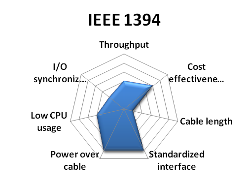
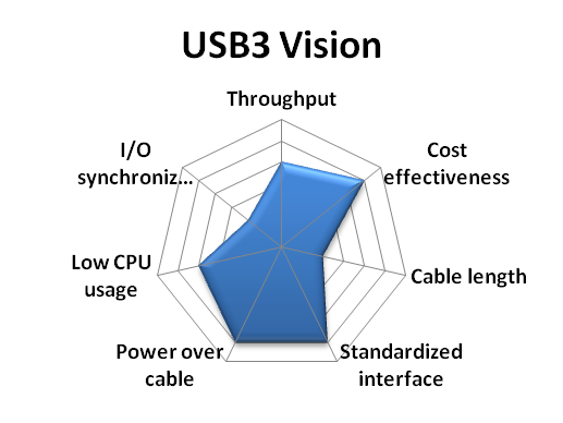
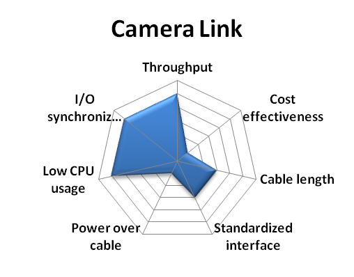
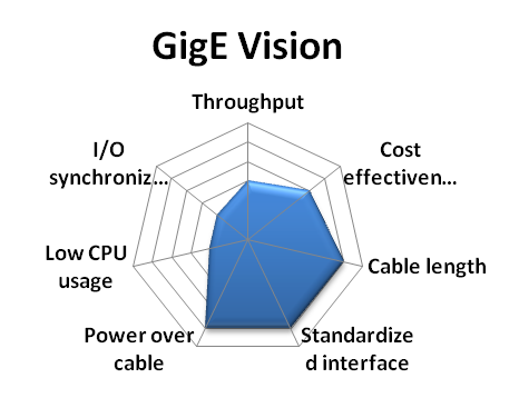
Figure 3.1 Vision camera buses comparison (Source: National Instruments white paper [Na13].
At the time of writing, the accompanying software for this course was primarily written in Matlab. If readers wish to collect their own data sets using our software, we recommend obtaining a camera supported by the Image Acquisition Toolbox for Matlab. Note that this toolbox supports products from a variety of vendors, as well as any DCAM-compatible FireWire camera or webcam with a Windows Driver Model (WDM) or Video for Windows (VFW) driver. For FireWire cameras the toolbox uses the CMU DCAM driver [CMU]. Alternatively, we encourage users to write their own image acquisition tools using standard libraries as OpenCV or SimpleCV. OpenCV has a variety of ready-to-use computer vision algorithms---such as camera calibration---optimized for several platforms, including Windows, Mac OS X, Linux, and Android; which can be accessed in C++, Java, and Python. SimpleCV is a high-level framework, with a faster learning curve, for developing computer vision software in Python.
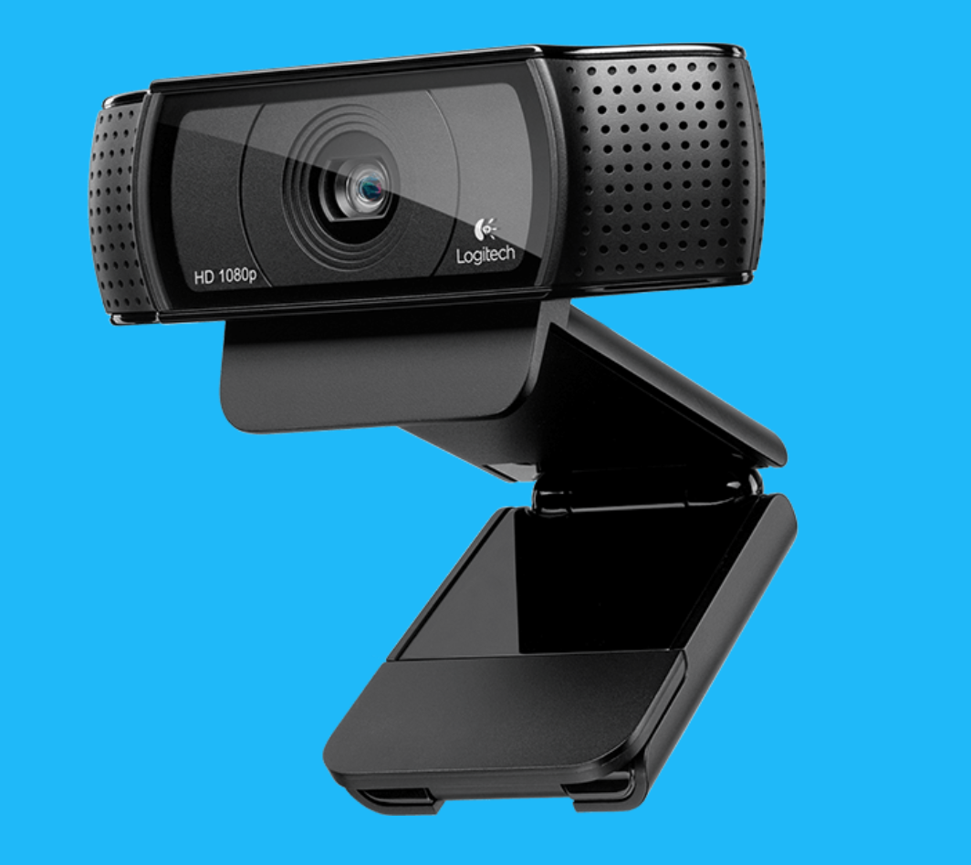
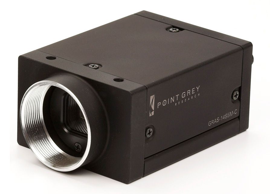
Figure 3.2 Recommended cameras for course projects: (Left) Logitech HD Pro Webcam C920; (Right) Point Grey Grasshopper IEEE-1394b (without lens)
Calibration Methods and Software
Camera Calibration Methods
Camera calibration requires estimating the parameters of the general pinhole model presented in Section General Pinhole. This includes the intrinsic parameters, being focal length, principal point, and the scale factors, as well as the extrinsic parameters, defined by a rotation matrix and translation vector mapping between the world and camera coordinate systems. In total, 11 parameters (5 intrinsic and 6 extrinsic) must be estimated from a calibration sequence. In practice, a lens distortion model must be estimated as well. We recommend the reader review [HZ04] or [MSKS05] for an in-depth description of camera models and calibration methods.
At a basic level, camera calibration requires recording a sequence of images of a calibration object, composed of a unique set of distinguishable features with known 3D displacements. Thus, each image of the calibration object provides a set of 2D-to-3D correspondences, mapping image coordinates to scene points. Naively, one would simply need to optimize over the set of 11 camera model parameters so that the set of 2D-to-3D correspondences are correctly predicted (i.e., the projection of each known 3D model feature is close to its measured image coordinates).
Many methods have been proposed over the years to solve for the camera parameters given such correspondences. In particular, the factorized approach originally proposed Zhang [Zha00] is widely-adopted in most community-developed tools. In this method, a planar checkerboard pattern is observed in two or more orientations (see Figure 3.3). From this sequence, the intrinsic parameters can be separately solved. Afterwards, a single view of a checkerboard can be used to solve for the extrinsic parameters. Given the relative ease of printing 2D patterns, this method is commonly used in computer graphics and vision publications.
Recommended Software
A comprehensive list of calibration software is maintained by Bouguet on the Camera Calibration Toolbox website. An alternative camera calibration package is the Matlab Camera Calibration Toolbox. Otherwise, OpenCV replicates many of its functionalities, while supporting multiple platforms. A CALTag checkerboard and software is yet another alternative. CALTag patterns are designed to provide features even if some checkerboard regions are occluded. we will use this feature in Section Turntable Calibration to calibrate a turntable.
Although calibrating a small number of cameras using these tools is straightforward, calibrating a large network of cameras is a relatively challenging problem. If your projects lead you in this direction, we suggest to consider the self-calibration toolbox [SMP05], or a new toolbox based on a feature-descriptor pattern [LHKP13] instead. The former, rather than using multiple views of a planar calibration object, detects a standard laser point being translated through the working volume and correspondences between the cameras are automatically determined from the tracked projection of the pointer in each image. The latter, creates a pattern using multiple SIFT/SURF features at different scales which can be automatically detected. In contrast with the checkerboard approach, features can be uniquely identified---similar to CALTag cells---even when partial views of the pattern are available due to limited intersection of the multiple cameras field of view.
Calibration Procedure
In this section we describe, step-by-step, how to calibrate your camera using the Camera Calibration Toolbox for Matlab. We also recommend reviewing the detailed documentation and examples provided on the toolbox website. Specifically, new users should work through the first calibration example and familiarize themselves with the description of model parameters (which differ slightly from the notation used in these notes).
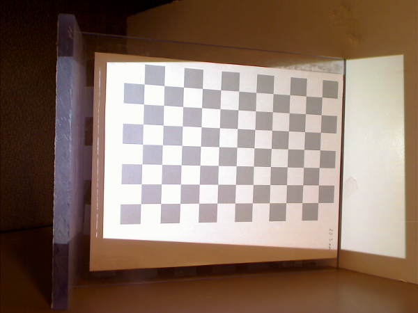
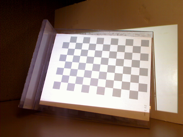
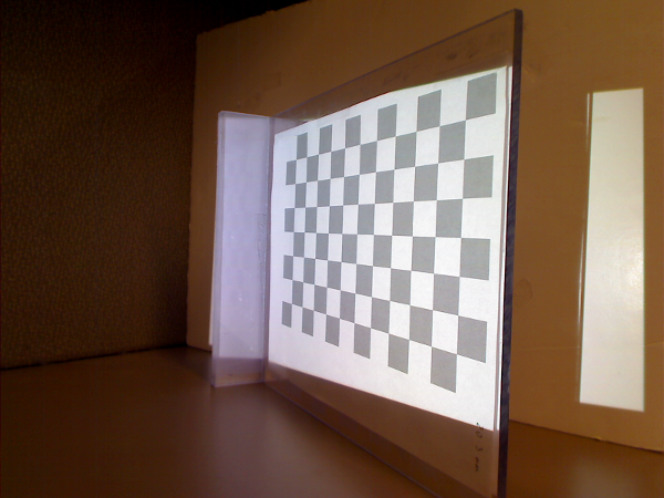
Figure 3.3 Camera calibration images containing a checkerboard with different orientations throughout the scene.
Begin by installing the toolbox, available for download at the Caltech Camera Calibration software website. Next, construct a checkerboard target. Note that the toolbox comes with a sample checkerboard image; print this image and affix it to a rigid object, such as piece of cardboard or textbook cover. Record a series of 10--20 images of the checkerboard, varying its position and pose between exposures. Try to collect images where the checkerboard is visible throughout the image, and specially, the checkerboard must cover a large region in each image.
Using the toolbox is relatively straightforward. Begin by adding the toolbox to your Matlab path by selecting \(\textsf{File} \rightarrow \textsf{Set Path...}\). Next, change the current working directory to one containing your calibration images (or one of our test sequences). Type \(\texttt{calib}\) at the Matlab prompt to start. Since we are only using a few images, select \(\textsf{Standard (all the images are stored in memory)}\) when prompted. To load the images, select \(\textsf{Image names}\) and press return, then \(\texttt{j}\) (JPEG images). Now select \(\textsf{Extract grid corners}\), pass through the prompts without entering any options, and then follow the on-screen directions. The default checkerboard has 30mm\(\times\)30mm squares but the actual dimensions vary from printer to printer, you should measure your own checkerboard and use those values instead. Always skip any prompts that appear, unless you are more familiar with the toolbox options. Once you have finished selecting corners, choose \(\textsf{Calibration}\), which will run one pass though the calibration algorithm. Next, choose \(\textsf{Analyze error}\). Left-click on any outliers you observe, then right-click to continue. Repeat the corner selection and calibration steps for any remaining outliers (this is a manually-assisted form of bundle adjustment). Once you have an evenly-distributed set of reprojection errors, select \(\textsf{Recomp. corners}\) and finally \(\textsf{Calibration}\). To save your intrinsic calibration, select \(\textsf{Save}\).
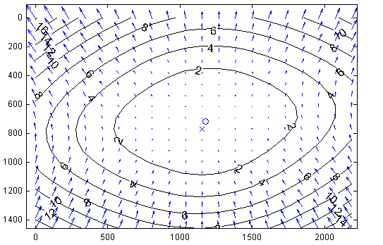
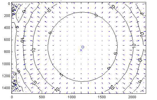
Figure 3.4 Camera calibration distortion model. (Left) Tangential Component. (Right) Radial Component. Sample distortion model of the Logitech C920 Webcam. The plots show the center of distortion \(\times\) at the principal point, and the amount of distortion in pixel units increasing towards the border.
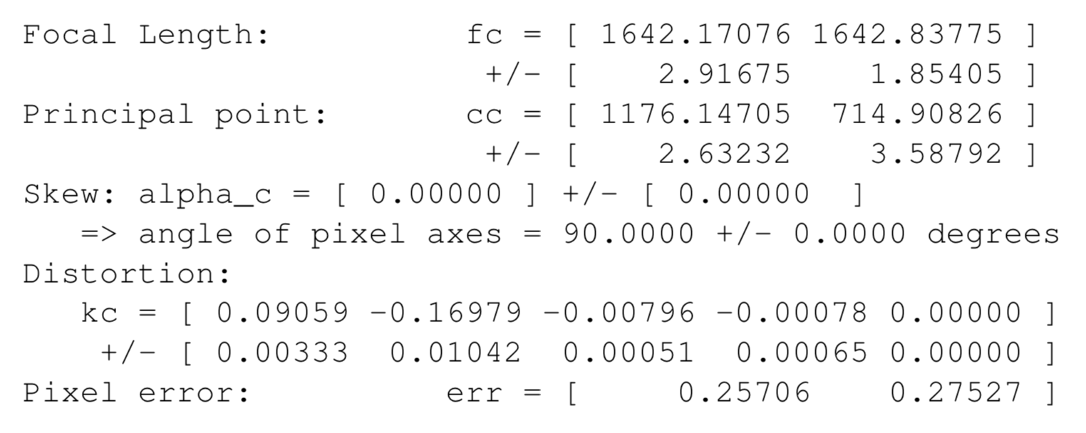
From the previous step you now have an estimate of how pixels can be converted into normalized coordinates (and subsequently optical rays in world coordinates, originating at the camera center). Note that this procedure estimates both the intrinsic and extrinsic parameters, as well as the parameters of a lens distortion model. Typical calibration results, illustrating the lens distortion model is shown in Figure 3.4. The actual result of the calibration is displayed below as reference.
Logitech C920 Webcam sample calibration result:
Projector Calibration
We now turn our attention to projector calibration. Following the conclusions of Chapter The Mathematics of Optical Triangulation, we model the projector as an inverse camera (i.e., one in which light travels in the opposite direction from usual). Under this model, calibration proceeds in a similar manner as with cameras, where correspondences between 3D points world coordinates and projector pixel locations are used to estimate the pinhole model parameters. For camera calibration, we use checkerboard corners as reference world points of known coordinates which are localized in several images to establish pixel correspondences. In the projector case, we will project a known pattern onto a checkerboard and to record a set of images for each checkerboard pose. The projected pattern is later decoded from the camera images and used to convert from camera coordinates to projector pixel locations. This way, checkerboard corners are identified in the camera images and, with the help of the projected pattern, their locations in projector coordinates are inferred. Finally, projector-checkerboard correspondences are used to calibrate the projector parameters as it is done for cameras. This calibration method is described with detail in [MT12] and implemented as an opensource calibration and scanning tool. We will use this software for projector and camera calibration when working with structured light scanners in Chapter 3D Scanning with Structured Light. A step-by-step guide of calibration process is given below in Section Projector Calibration.
Projector Selection and Interfaces
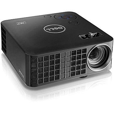
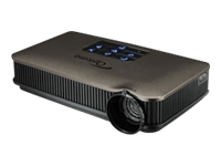
Figure 3.5 Recommended projectors for course projects: (Left) Dell M110 DLP Pico Projector, (Right) Optoma PK320 Pico Pocket Projector.
Almost any digital projector can be used in your 3D scanning projects, since the operating system will simply treat it as an additional display. However, we recommend at least a VGA projector, capable of displaying a \(640\times 480\) image. For building a structured lighting system select a camera with equal (or higher) resolution than the projector. Otherwise, the recovered model will be limited to the camera resolution. Additionally, those with DVI or HDMI interfaces are preferred for their relative lack of analogue to digital conversion artifacts.
The technologies used in consumer projectors have matured rapidly over the last decade. Early projectors used an LCD-based spatial light modulator and a metal halide lamp, whereas recent models incorporate a digital micromirror device (DMD) and LED lighting. Commercial offerings vary greatly, spanning large units for conference venues to embedded projectors for mobile phones. A variety of technical specifications must be considered when choosing the best projector for your 3D scanning projects. Variations in throw distance (i.e., where focused images can be formed), projector artifacts (i.e., pixelization and distortion), and cost are key factors.
Digital projectors have a tiered pricing model, with brighter projectors costing significantly more than dimmer ones. At the time of writing, a portable projector with output resolution of \(1280\times 800\) and \(100\)--\(500\) lumens of brightness can be purchased for around \(\$300\)--\(\$500\) USD. Examples are the Optoma and Dell Pico projectors shown in Figure 3.5 commonly used by students because of their convenient small size and high contrast.
When considering projectors it is important to distinguish between their native and output resolutions. Native resolution refers to the number of pixels in the projection device (i.e. number of micromirrors in DLPs arrays), whereas, the output resolution is the screen size reported to the operating system. Ideally, we want both to be the same so that images sent by the operating are displayed by the projector at the same resolution. However, many portable projectors use Texas Instruments DLP Pico DMDs where projector pixels are rotated \(45^{\circ}\) as shown in Figure 3.6. In this configuration the pixel density in the horizontal and vertical directions are different and images generated by the computer are resampled to match the DMD elements. We have used pico projectors in structured-light scanners successfully but the native resolution has to be considered to decide the maximum resolution of the projected patterns.
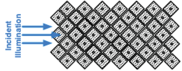
Figure 3.6 TI DLP .45in Pico Projectors diamond pixel configuration.
While your system will treat the projector as a second display, your development environment may or may not easily support fullscreen display. For instance, Matlab does not natively support fullscreen display (i.e., without window borders or menus). One solution is to use Java display functions integrated in Matlab. Code for this approach is available online. Unfortunately, we found that this approach only works for the primary display. Another common approach is to split image acquisition and data processing in two separate programs and use standard software (i.e. as provided by camera manufacturers) to capture and save images, and to program your scanning tool to read images from a permanent storage. This approach is used by the Caltech Camera Calibration software. Finally, for users working outside of Matlab, we recommend controlling projectors through OpenGL.
Calibration Software and Procedure
Projector calibration has received increasing attention, in part driven by the emergence of low-cost digital projectors. As mentioned at several points, a projector is simply the inverse of a camera, wherein points on an image plane are mapped to outgoing light rays passing through the center of projection. As in Section Camera Calibration Methods, a lens distortion model can augment the basic general pinhole model presented in The Mathematics of Optical Triangulation. In this section we will use the Projector-Camera Calibration software to calibrate both projector and camera, intrinsic and extrinsic parameters, including radial distortion coefficients. This software is built for Windows, Linux, and Mac OS X, and source code is available too.
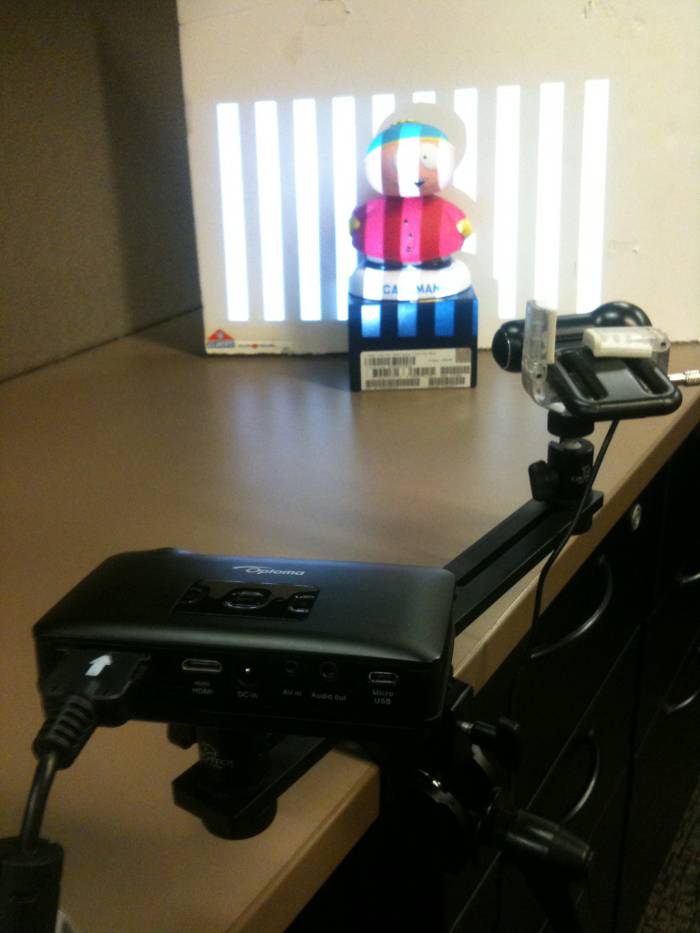
Figure 3.7 Sample setup of a structured light scanner. A projector and camera are placed at similar height with a horizontal translation in stereo configuration. In this particular case, the camera is much forward than the projector to compensate between their different field of view.
Begin by downloading the software for your platform and setting up your projector and camera in the scanning position. Once calibrated, projector and camera have to remain at fix positions, and their lens settings unchanged (e.g. focus, zoom) for the calibration to remain valid. The general recommendation is to place them with some horizontal displacement, too much displacement will provide little overlap between projector and camera images, too few displacement will produce a lot of uncertainty for triangulation, try to find some intermediate position, see Figure Figure 3.7 as example. A checkerboard pattern is required for calibration.
Run the software and click the \(\textsf{Capture...}\) button to open a preview window, Figure 3.8. Select your projector screen and your camera using the combo boxes, then check \(\textsf{Preview}\) to activate the projector. Click \(\textsf{Prev}\) and \(\textsf{Next}\) buttons to navigate the projected pattern sequence as desired. Use the camera live view to make sure camera and projector view points are correct. Note that only cameras supported by OpenCV will be recognized by the software; if your camera happens to not be in this group, you can still use the tool for calibration but you will have to project and capture the images with an external software, and use the tool only for calibration. Refer to the software website for more details.
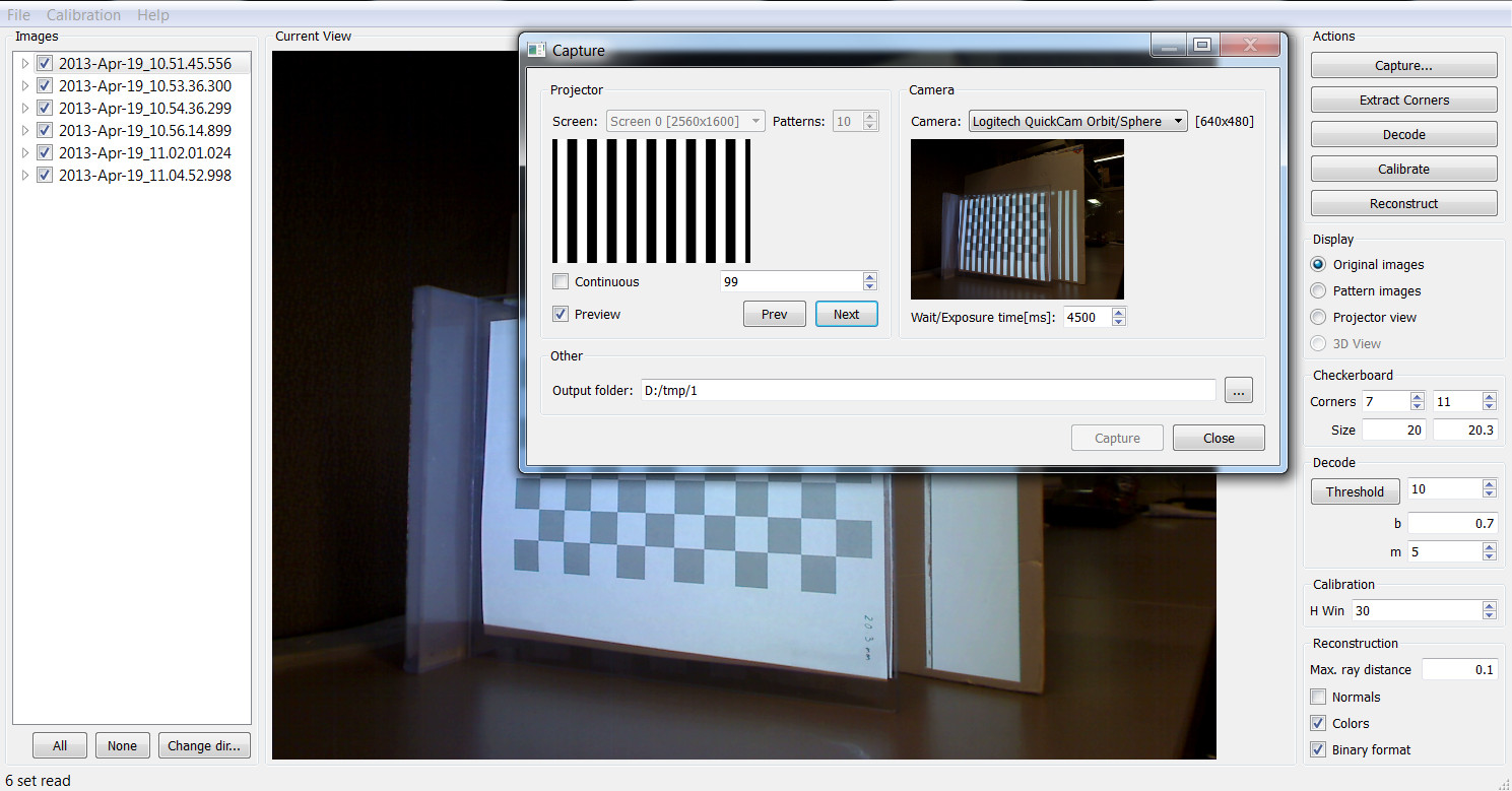
Figure 3.8 Projector-Camera Calibration software main screen and capture window.
Place the calibration checkerboard in the scene in such a way that all its cells are visible in the camera and illuminated by the projector. Uncheck \(\textsf{Preview}\) and press \(\textsf{Capture}\). The software will project and capture a sequence of images. The checkerboard has to remain static at this time. The image output folder can be changed prior beginning, but it must not be changed after the first capture. Repeat the capture procedure several times to collect sequences with the checkerboard at different positions and orientations. Close the capture window to return to the main screen.
The main screen will display a list with the different sequences captured, which can be browsed to see any of the images. If images were captured with an external tool, or with this tool but at a different time, you can select their location by clicking \(\textsf{Change dir..}\). Count the internal number of corners of your checkerboard and fill the boxes labeled as \(\textsf{Corners}\), also measure them in millimeters, or your unit of choice, and enter their dimensions in the \(\textsf{Size}\) boxes. Now you are ready for calibration, click \(\textsf{Calibrate}\). The program will automatically detect the checkerboard corners, decode the projected sequences, and run the calibration. The final result will be displayed as text and saved to a file. The main screen contains other parameters and buttons that can be used to debug errors or to change the default decoding options, they will not be covered here but feel free to read the documentation and modify them to improve your results.