The Laser Slit 3D Scanner
In this chapter we describe how to build the classic desktop Laser Slit 3D Scanner consisting of a single digital camera, a laser line projector, and a manual or motorized turntable. Specifically, we will describe how to setup the scanner using inexpensive elements, and we will describe its operating principle and the mathematics that allow to compute the 3D shape of an object being scanned.
Description
The Laser Slit 3D Scanner is an active line scanner, meaning that it uses active illumination---the laser line projected onto a scene---and that it recovers a single line of points from each captured frame. Active illumination permits to scan objects more or less independently of their surface color or texture, which is an important advantage over passive methods which have difficulty in recovering constant color regions. On the other hand, a single line is captured at each time and it is necessary to move either the scanner or the object to acquire additional points and incrementally build a 3D model. In our case, we decided to put the target object onto an inexpensive turntable which is rotated manually in order to create a \(360^{\circ}\) model. Some users may prefer to use a computerized turntable controlled by a stepper motor for more automation or may want to do other variations to the suggested setup. The mathematics and methods discussed here will be applicable with little or no modification to many of these variations.
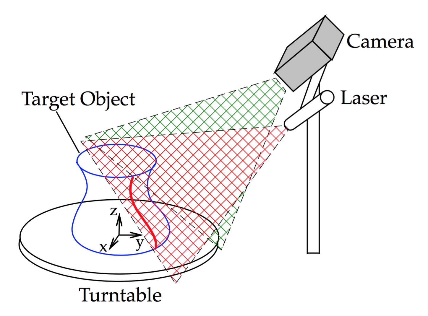
Figure 4.1 Laser Slit 3D Scanner setup
The scanner is setup as shown in Figure 4.1. The camera is fixed on a side, elevated from the turntable plane, and looking down to the turntable center. The optimal orientation and distance depends on the camera field-of-view and the size of scanning volume. The general guideline is that most of the turntable surface must be visible when there is no object on it, and the bottom and top of the object being scanned must be visible too when sitting on the turntable. It is not recommended to put the camera farther than required because the image regions looking at neither the turntable nor the target object will not be used by the scanner. The Laser Line Generator must be placed on a side of the camera and with similar orientation, it is recommended that it passes through the turntable center point and be orthogonal to the turntable plane. Figure 4.2 shows the materials we have used in our setup: a 650nm AixiZ \(38^{\circ}\) Line Generator, a Logitech HD Pro Webcam C920, and a manually controlled turntable.
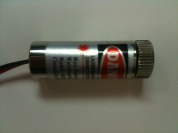
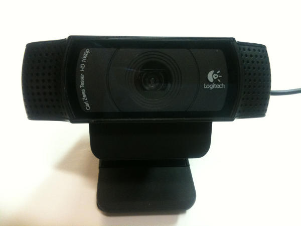
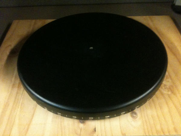
Figure 4.2 Materials: (Left) 650nm AixiZ \(38^{\circ}\) Line Generator. (Center) Logitech HD Pro Webcam C920. (Right) Manual turntable.
We will set the world coordinate system at the turntable center of rotation, with the \(xy\)-plane on the turntable and the \(z\)-axis pointing up, see Figure 4.1. Prior to scanning, we need to calibrate the camera intrinsic parameters and the location of both the camera and light plane generated by the laser in respect to the world coordinate system. The turntable center of rotation must be calibrated too. At scanning time, the light plane generated by the laser is invisible in the air but we can see some of its points when the light hits a surface, they will have the color of the projected light (red in our case). These points can be detected in an image captured by the camera and its 3D location is found as the intersection of a ray beginning at the camera center, passing through the corresponding image pixel, and the plane of light (known), Figure 4.3. The location of the points recovered from each image must be rotated through the \(z\)-axis to undo the current turntable rotation angle.
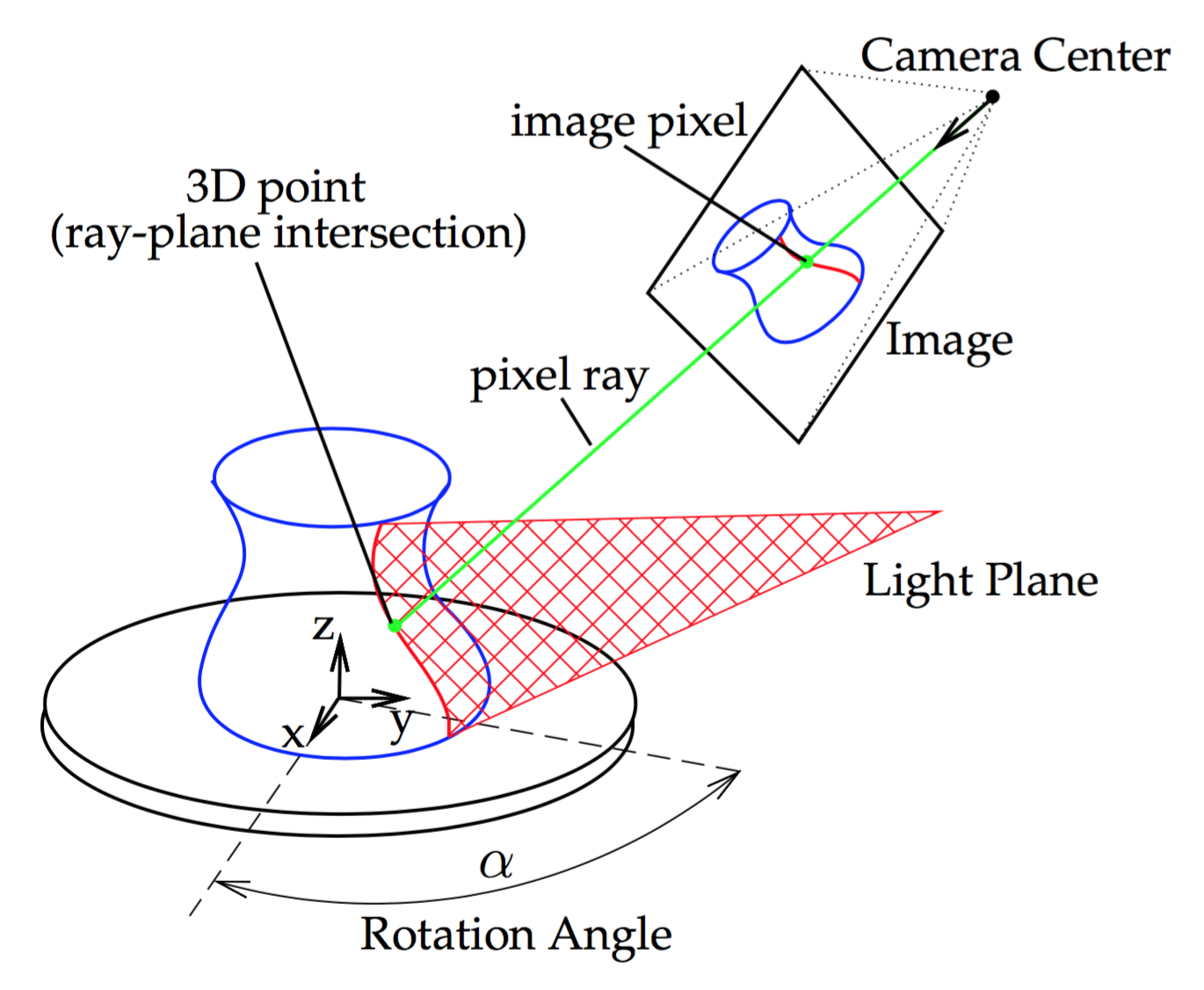
Figure 4.3 Laser Slit 3D Scanner setup
Turntable calibration
A computer controlled turntable will provide us with the current
rotation angle that corresponds to the stepper motor current
rotation. Sometimes, as in the case of a manual turntable, that
information is not available and the rotation must be computed from
the current image. We will do so with the help of a CALTag
checkerboard [AHH10] pasted flat
on the turntable surface. The CALTag checkerboard assigns a unique
code to each checkerboard cell which is used to identify the visible
cells in an image even when a region of the checkerboard is
occluded. We need this property because the target object sitting on
top the turntable will occlude a large region of the CALTag. The
corners of the visible checkerboard cells is a set of points rotating
together with the turntable and will allow us to compute a rotation
angle for each captured image.
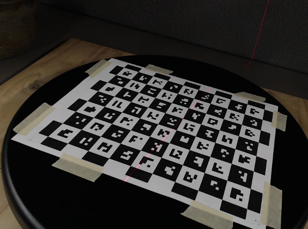
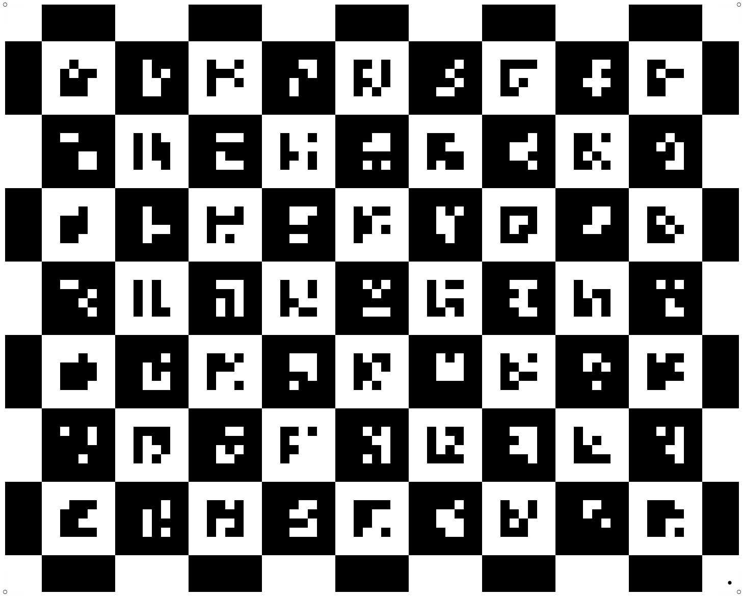
Figure 4.4 (Left) A CALTag checkerboard pasted on the turntable surface helps to recover the current rotation angle. (Right) Sample CALTag pattern.
At this point we assume the camera is calibrated and a set of images of the turntable at different rotations was captured. In addition, a set of 3D points on the turntable plane was identified in each image. Points coordinates are in reference to a known coordinate system chosen by the user. We will show how to find the unknown center of rotation and the rotation angle of the turntable for each image. In the current example, we align the coordinate system with the checkerboard and we identify the checkerboard and turntable planes with the plane \(z=0\).
Camera extrinsics
The first step is to find the pose of the camera for each image in reference to the known coordinate system. At this point we will compute a rotation matrix \(R\) and a translation vector \(T\) for each image independently of the others, such that a point \(p\) in the reference system projects to a pixel \(u\), that is
\begin{equation} \label{eq:turntable:proj} \lambda u = K (R p + T) \end{equation}
\begin{equation} \label{eq:turntable:ext0} R=\begin{bmatrix} r_{11}&r_{12}&r_{13}\\ r_{21}&r_{22}&r_{23}\\ r_{31}&r_{32}&r_{33} \end{bmatrix}, \ T=\begin{bmatrix}T_x\\T_y\\T_z\end{bmatrix} \end{equation}
where \(u\), \(p\), and \(K\) are known. Point \(p = [p_x, p_y, 0]^T\) is in the checkerboard plane and \(u = [u_x, u_y, 1]^T\) is expressed in homogenous coordinates. We define \(\tilde{u}=K^{-1}u\) and rewrite Equation \ref{eq:turntable:proj} as follows
\begin{equation} \label{eq:turntable:ext1} [0,0,0]^T = \tilde{u} \times (\lambda \tilde{u}) = \tilde{u} \times (R p + T) \end{equation}
\begin{equation}\label{eq:turntable:ext2} \tilde{u} \times \begin{bmatrix}r_{11}p_x+r_{12}p_y+T_x\\r_{21}p_x+r_{22}p_y+T_y\\r_{31}p_x+r_{32}p_y+T_z\end{bmatrix} = \begin{bmatrix}0\\0\\0\end{bmatrix} \end{equation}
\begin{equation}\label{eq:turntable:ext3} \begin{bmatrix} \ \ \ \ -(r_{21}p_x+r_{22}p_y+T_y)&+&\tilde{u}_y(r_{31}p_x+r_{32}p_y+T_z)\\ \ \ \ \ \ \ \ (r_{11}p_x+r_{12}p_y+T_x)&+&\tilde{u}_x(r_{31}p_x+r_{32}p_y+T_z)\\ -\tilde{u}_y(r_{11}p_x+r_{12}p_y+T_x)&+&\tilde{u}_x(r_{21}p_x+r_{22}p_y+T_y) \end{bmatrix} = \begin{bmatrix}0\\0\\0\end{bmatrix}. \end{equation}
Equation \ref{eq:turntable:ext3} provides 3 equations but only 2 of them are linearly independent. We select the first two equations and we group the unknowns in a vector \(X = [r_{11},r_{21},r_{31},r_{12},r_{22},r_{32},T_x,T_y,T_z]^T\)
\begin{equation}\label{eq:turntable:ext4} \begin{bmatrix} 0&-p_x&+\tilde{u}_y p_x & 0&-p_y&+\tilde{u}_y p_y & 0&-1&+\tilde{u}_y\\ p_x& 0&-\tilde{u}_x p_x &p_y& 0&-\tilde{u}_x p_y & 1& 0&-\tilde{u}_x \end{bmatrix} X = \begin{bmatrix}0\\0\end{bmatrix}. \end{equation}
Until now we have considered a single point \(p\); in general, we will have a set of points~\(\smash\{p_i|i:1\ldots n\}\) for each image. Note that the number \(n\) of points visible will change from image to image. We use all the points to build a single system of the form \(AX=0\) where \(A \in \mathbb{R}^{2n\times 9}\) contains 2 rows as in Equation \ref{eq:turntable:ext4} for each point \(p_i\) stacked together, and we solve
\begin{equation}\label{eq:turntable:ext5} \hat{X} = arg\min_X ||AX||,\ \ \ \text{s.t.} \ \ ||X|| = 1 \end{equation}
We constrain the norm of X in order to get a non-trivial solution. Vector \(X\) has 8 degrees of freedom, thus, matrix \(A\) must be rank 8 so that a unique solution exists. Therefore, we need at least 4 non-collinear points in order to get a meaningful result. After solving for \(\hat{X}\) we need to rebuild \(R\) as a rotation matrix.
\begin{equation}\label{eq:turntable:ext6} \hat{r_1} = [r_{11},r_{21},r_{31}]^T, \ \hat{r_2} = [r_{21},r_{22},r_{23}]^T, \ \hat{T} = [T_x,T_y,T_z]^T \end{equation}
\begin{equation}\label{eq:turntable:ext7} r_1 = \frac{\hat{r_1}}{||\hat{r_1}||}, \ r_3 = \frac{\hat{r_1}}{||\hat{r_1}||}\times\frac{\hat{r_2}}{||\hat{r_2}||}, \ r_2 = r_3 \times r_1 \end{equation}
\begin{equation}\label{eq:turntable:ext8} R = \begin{bmatrix}r_1&r_2&r_3\end{bmatrix}, \ T = \hat{T} \end{equation}
Figure 4.5 shows the supplied software running the camera extrinsics computation as described here.
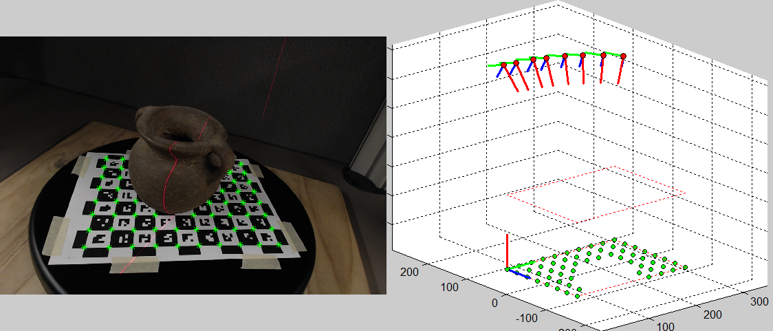
Figure 4.5 Screenshot of the supplied software running camera extrinsics computation. (Left) Image being processed: identified CALTag corners displayed in green. (Right) 3D view: CALTag corners shown in green below, cameras displayed above with their \(z\)-axis on red, the reference coordinate system was set at the origin of the checkerboard.
Center of rotation and rotation angle
In the previous section we showed how to estimate \(R_k\) and \(T_k\) for each of the \(N\) cameras independently. Now, we will use the fact that the turntable rotates in a plane and has a single degree of freedom to improve the computed camera poses. We begin finding the center of rotation \(q=[q_x,q_y,0]^T\) in the turntable plane which must satisfy the projection equations as any other point
\begin{equation} \lambda_k \tilde{u}_k = R_k q + T_k \end{equation}
By definition of rotation center its position remains unchanged before and after the rotation, this observation allow us to define \(Q\equiv\lambda_k \tilde{u}_k,\ \forall k\), and write
\begin{equation} R_k q + T_k = Q \end{equation}
\begin{equation} \begin{bmatrix}R_1&-I\\R_2&-I\\\vdots&\vdots\\R_N&-I\end{bmatrix} \begin{bmatrix}q\\Q\end{bmatrix} = \begin{bmatrix}-T_1\\-T_2\\\vdots\\-T_N\end{bmatrix} \ \Rightarrow\ AX=b \end{equation}
\begin{equation} \hat{X} = arg\min_X ||AX-b|| \end{equation}
In order to fix \(q_z=0\), we skip the third column in the rotation matrices reducing \(A\) to 5 columns and changing \(X = [q_x,q_y,Q_x,Q_y,Q_z]^T\).
Let be \(\alpha_i\) the rotation angle of the turntable in image \(i\),
then for every \(1\leq k
\begin{equation}
R_k^T R_j = \begin{bmatrix}
\cos(\alpha_j-\alpha_k)&-\sin(\alpha_j-\alpha_k)&0\\
\sin(\alpha_j-\alpha_k)&\ \ \cos(\alpha_j-\alpha_k)&0\\
0&0&1\\
\end{bmatrix}
\end{equation}
The turntable position in the first image is designated as the origin:
\(\alpha_1=0\). We get an approximate value for each other \(\alpha_k\)
by reading the values \(\cos\alpha_k\) and \(\sin\alpha_k\) from \(R_1^T
R_k\) and setting
\begin{equation}
\alpha_k = \tan^{-1}\biggl(\frac{\sin\alpha_k}{\cos\alpha_k}\biggr)
\end{equation}
Figure 4.6 shows the center of rotation
obtained with this method drawn on top of an input image and its
corresponding 3D view.
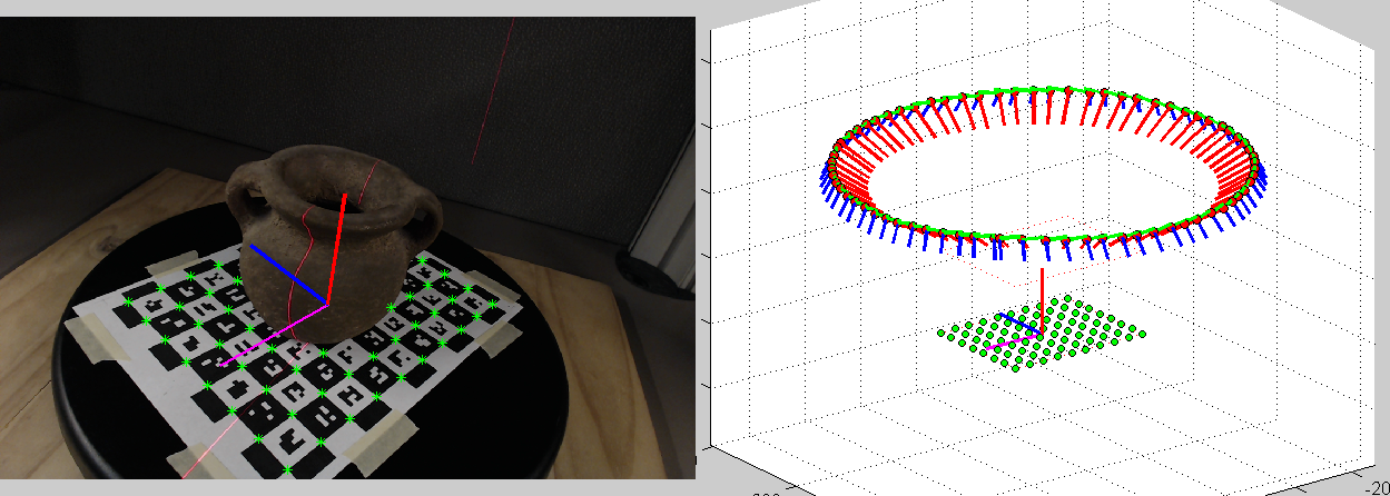
Figure 4.6
Center of rotation. (Left) Camera image: center of rotation
drawn on top. (Right) 3D view: world coordinate system at the center
of the rotation.
Global Optimization
The final step in turntable calibration is to refine the values of all the parameters using a global optimization. The goal is to minimize the reprojection error of the detected points in the images
\begin{equation} E(q_x,q_y,R_1,o_1,\alpha_2,\ldots,\alpha_N) = \sum_{k=1}^N \sum_{i\in J_k} ||u_k^i - \Pi( K R_1 R_{\alpha_k}(p_i-o_k) )||^2 \end{equation}
where
\begin{equation} R_{\alpha_k} = \begin{bmatrix} \cos(\alpha_k)&-\sin(\alpha_k)&0\\ \sin(\alpha_k)&\ \ \cos(\alpha_k)&0\\ 0&0&1\\ \end{bmatrix}, \ o_k = R_{\alpha_k}^T(o_1-q) + q,\ \ \forall k>1, \end{equation}
and
\begin{equation} \Pi(x,y,z) = (x/z, y/z) \end{equation}
\(J_k\) is the subset of checkerboard corners visible in image \(k\), \(\alpha_1 = 0\), and \(u_k^i\) is the pixel location corresponding to \(p_i\) in image \(k\). We begin the optimization with the values \(q\), \(R_1\), \(o_1=-R_1^T T_1\), and \(\alpha_k\) found in the previous sections which are close to the optimal solution.
Image Laser Detection
In this section we show how to detect the laser slit in the captured images. A common approach to detection is to compare an image where the laser is seen with a reference image captured while the laser is off. That approach is appropriate for a scanner setup where the camera and the object remains static while the laser changes location. Detection is done by subtracting the intensity in the new image with the reference intensity and searching the pixels where a significance change is observed. This method works independently of the laser color, would work even when color images are not available, it is computationally efficient, and most importantly, it is tuned to the current scene and illumination, because a new reference image is captured for each new scanning. However, the method is not applicable if a reference image is not available, or as in the case of the turntable where we would need as many reference images as turntable positions.
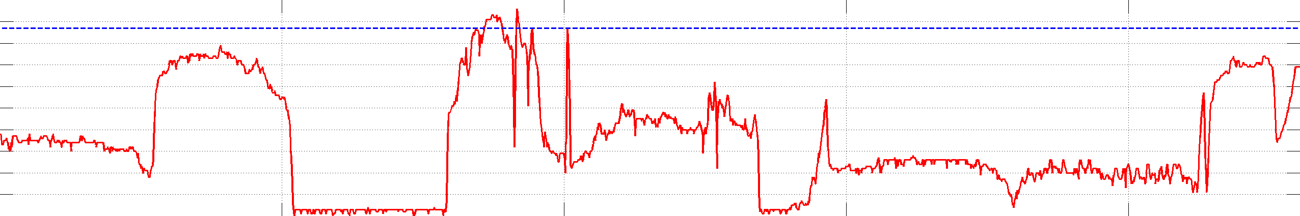
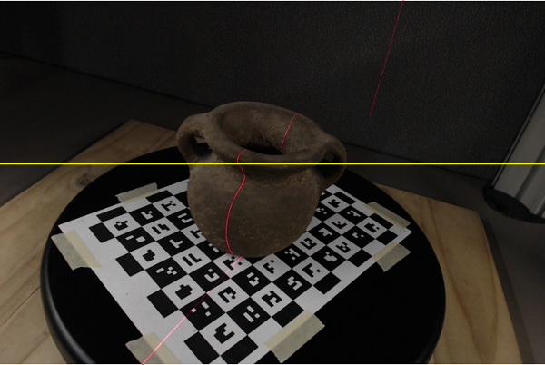
Figure 4.7 The plot shows the red channel intensity along the line in the image highlighted in yelow. The maximum value does not corresponds to the laser line.
In our scanner we will apply a laser detection algorithm that considers the laser color and it does work with a single image. In our case we used a red laser and we could expect to examine the image red channel and find a maximum at the laser location. This is not always true even if there are no other red points in the scene. For instance, Figure 4.7 shows a typical input image, without any red color visible besides the laser line, but the highlighted line contains many pixels with red intensity above the value at the laser location, indicated with a blue line in the plot. The reason is that red color is not the one with a high value in the red channel---white has high intensities in all channels. The property of red color is that it \emph{only} has a high intensity in the red channel. Based on this observation we will perform the detection in a channel difference image defined as
\begin{equation}\label{eq:turntable:Idiff} I_{diff} = I_r - \frac{I_g+I_b}{2} \end{equation}
where \(I_r\), \(I_g\), and \(I_b\) are the image red, green, and blue channels respectively. Figure 4.8 shows \(I_{diff}\) for the sample image. Now, there is a clear peak at the laser location.
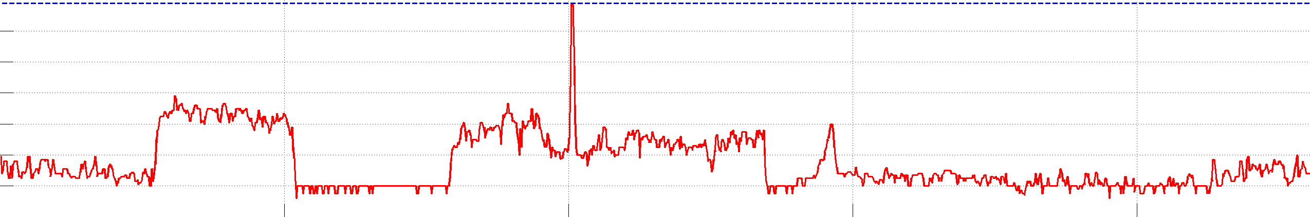
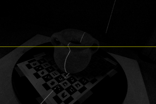
Figure 4.8 Channel difference. The image and plot show a clear peak at the laser line location.
Our detection algorithm involves computing the channel difference image with Equation \ref{eq:turntable:Idiff} and finding its maximum row by row. In general, we hope to find a single or no laser slit point in each row because we have oriented the laser line generator vertically. However, in rare occasions may appear more than one laser slit per line due to object discontinuities. For simplicity, we will consider only the one with maximum intensity.
Laser line generators made with a cylinder lens produce a Gaussian light distribution. In practice, cheap lenses have a profile not so well defined and the observed maximum will vary randomly in a range close to the line center, Figure 4.9. In order to compensate and make the estimation more stable from row to row, it is recommended to apply Gaussian smoothing in the horizontal direction prior to searching the maximum.
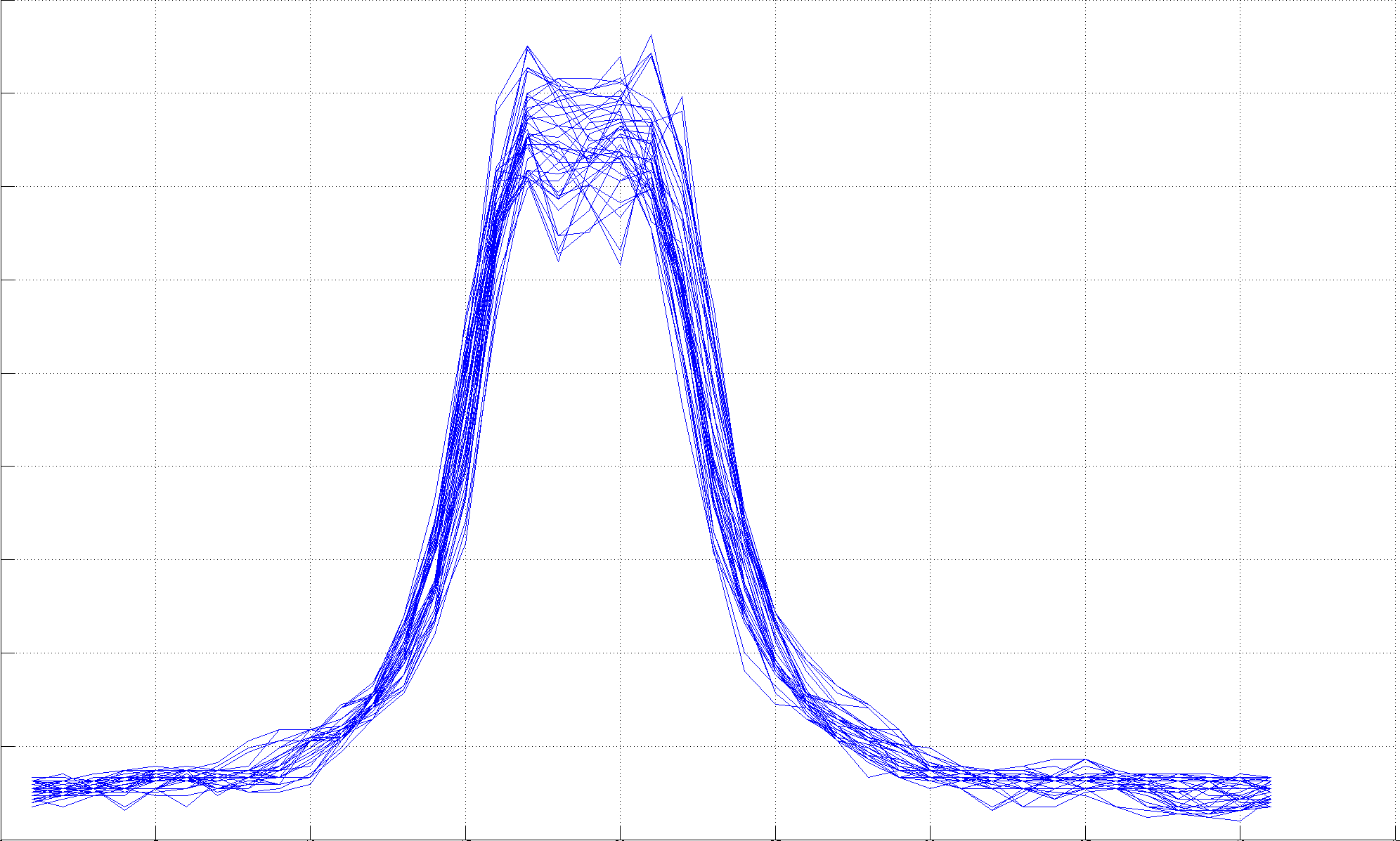
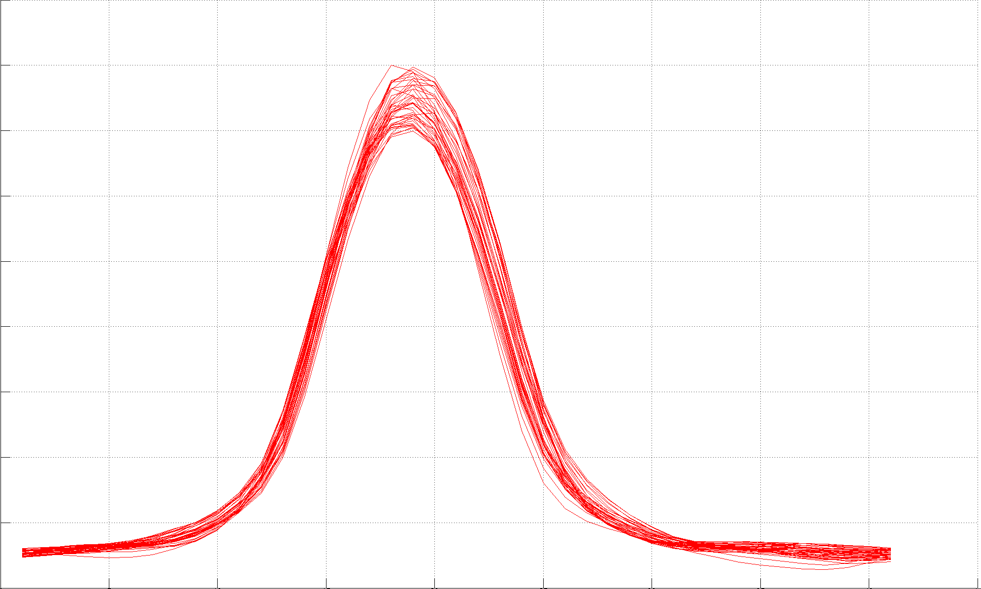
Figure 4.9 Laser line intensity plot of several image rows of similar color: (Left) there is no clear maximum at the peak center, (Right) the maximum is well localized after smoothing.
Figure 4.10 shows the result of the single image laser stripe detection described to the sample image.
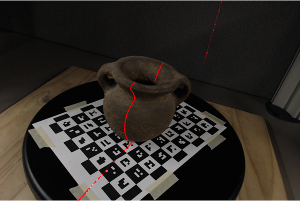
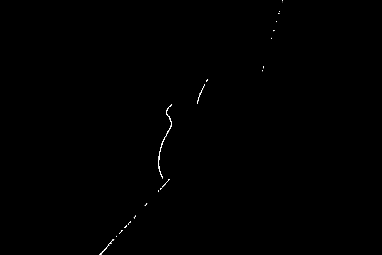
Figure 4.10 Laser detection result: (Top) detected points overlapped in red to input image, (Bottom) detection result mask.
Background detection
It is desirable to detect and exclude the background from the scanning process. Doing so saves computation on unwanted image regions, reduces detection errors, and produces a 3D model only with the object of interest. A pixel imaging a point on the turntable or the object sitting on top of it will be considered as foreground, all the other pixels are considered background. The set of foreground and background pixels are disjoint and the union of them contains the whole image. Additionally, a pixel location could be background in one image and foreground on a different one. Our goal is to compute the intersection of all images background pixels, that is, identify the pixel locations that are never foreground and we would like exclude from further processing.
By definition, a pixel location that is always background will have constant intensity. In reality, a background pixel will have little intensity variations due to the image sensor noise and small illumination changes. We can check this property by calculating the intensity variance of each pixel in the whole image set and label as background those with small variances.
Figure 4.11 (Left and Middle) verifies the constant property of background pixels visually. The background in the mean image is seen sharp, whereas, foreground pixels are blurred due to their changing intensities. Background pixels are close to zero (black) in the variance image. The detection result is displayed as a binary mask in Figure 4.11-(Right), foreground is shown in white.
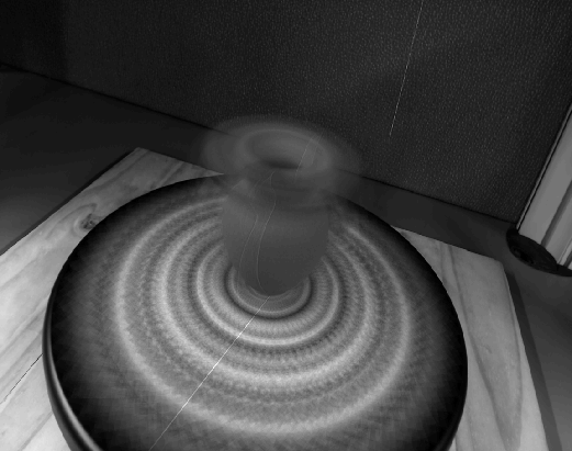
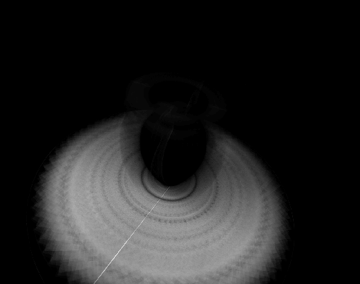
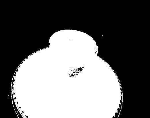
Figure 4.11 Background detection: (Left) mean intensity image, (Middle) variance intensity image, (Right) background mask result.
Plane of light calibration
We need to calibrate the location of the plane of light generated by the laser. The calibration consists in identifying some points we know belong to the plane and finding the best plane, in the least squares sense, that matches them. The projection of the laser line onto the turntable provides us with a set of such points, however, they are all in a straight line and define a pencil of planes rather a single one. An easy way to find additional points is to place a checkerboard plane onto the turntable and capture images at several rotations, Figure 4.12.
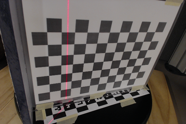
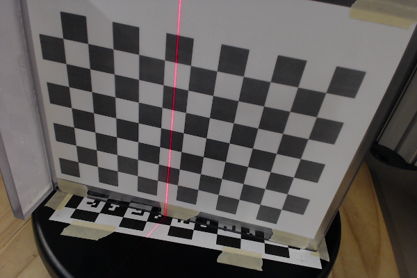
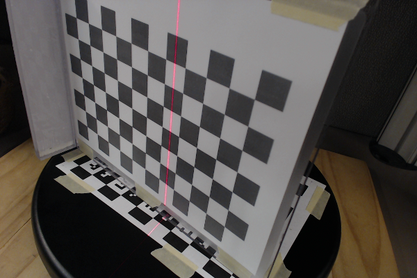
Figure 4.12 Light plane calibration: an extra plane is placed onto the turntable and is rotated to provide a set of non-collinear points.
The orientation of the camera with respect to the checkerboard plane is calculated with the method from Extrinsics section. The laser pixels are identified with the detection algorithm and they are triangulated using ray-plane intersection providing a set of 3D points on the checkerboard plane. We can choose to triangulate the laser points on the turntable plane too, which makes possible to calibrate with a single image. It is recommendable to capture additional images to have more samples of the light plane for a better calibration. In special, we would like samples at different depths in the scanning volume. Checkerboard images captured for the camera intrinsic calibration can be reused to calibrate the plane of light, this way no extra images are required. This idea is illustrated in Figure 4.13.
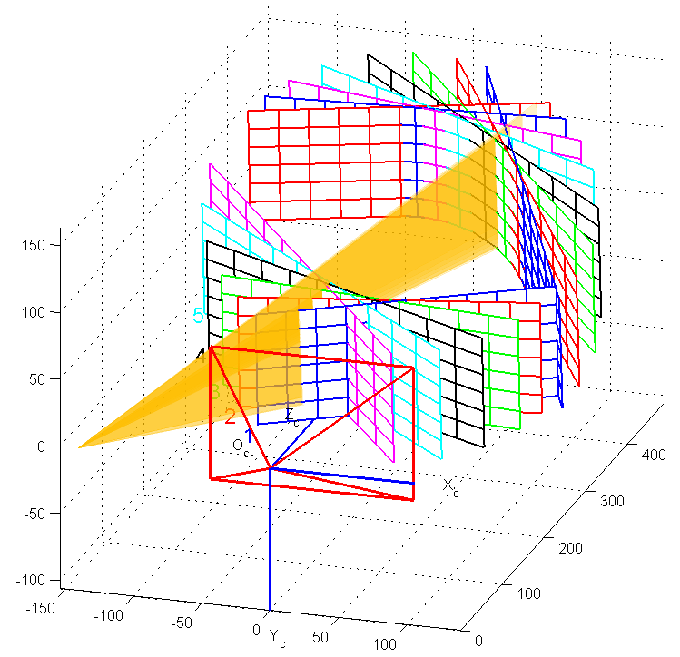
Figure 4.13 Light plane calibration result. A checkerdboard plane was placed on the turntable and images at several rotations were captured. Images are used first for camera calibration, and later for calibration of the light plane (shown in orange).
3D model reconstruction
At this point the system is fully calibrated: camera internal parameters, camera pose, world coordinate system, turntable rotation angle in each image, and the plane of light are all known. The last step is to identify the laser slits corresponding to the target object, triangulate them by ray-plane intersection with the light plane, and place the result in the world coordinate system by undoing the turntable rotation at each image. To generate only points in the model only foreground pixels are triangulated, and only the 3D points within the scanning volume are added to the model. The scanning volume is easily defined as the rectangular region of the turntable checkerboard and extending vertically in the direction of the \(z\)-axis by a user given height. Figure 4.14 shows the result output following the methods from this chapter and without any additional post-processing.
Figure 4.14 Laser Slit 3D Scanner result: (Top) 3D model in the sample software, (Bottom) 3D model output.